


Dates and times with lubridate package
- sam33frodon
- Jan 25, 2021
- 7 min read
library(lubridate)##
## Attaching package: 'lubridate'## The following objects are masked from 'package:base':
##
## date, intersect, setdiff, union1. BASICS
1.1. To get the current date or date-time
today()
## [1] "2021-01-25"
now()
## [1] "2021-01-25 12:19:09 EST"
1.2. Three ways to create a date/time:
From a string
From individual date-time components
From an existing date/time object
1.2.1. From a string
date_string = "2021-01-24" class(date_string)
## [1] "character"
ymd(date_string)
## [1] "2021-01-24"
mdy("January 21st, 2021")
## [1] "2021-01-21"
dmy("24-January-2021")
## [1] "2021-01-24"
These functions also take unquoted numbers. This is the most concise way to create a single date/time object, as you might need when filtering date/time data. ymd() is short and unambiguous:
ymd(20210124)
## [1] "2021-01-24"
ymd(20210103)
## [1] "2021-01-03"
ydm(20210103)
## [1] "2021-03-01"
To create a date-time, add an underscore and one or more of “h”, “m”, and “s” to the name of the parsing function:
ymd_hms("2021-01-24 23:18:59")
## [1] "2021-01-24 23:18:59 UTC"
mdy_hm("01/24/2021 08:01")
## [1] "2021-01-24 08:01:00 UTC"
1.2.2. From individual components
library(tidyverse) library(nycflights13)
flights %>%
    select(year, month, day, hour, minute) %>%
    head(10)

## # A tibble: 10 x 5 ##     year month   day  hour minute ##    <int> <int> <int> <dbl>  <dbl> ##  1  2013     1     1     5     15 ##  2  2013     1     1     5     29 ##  3  2013     1     1     5     40 ##  4  2013     1     1     5     45 ##  5  2013     1     1     6      0 ##  6  2013     1     1     5     58 ##  7  2013     1     1     6      0 ##  8  2013     1     1     6      0 ##  9  2013     1     1     6      0 ## 10  2013     1     1     6      0
To create a date/time from this sort of input, use make_date() for dates, or make_datetime() for date-times:
flights %>%
	select(year, month, day) %>%
	mutate(departure = make_datetime(year, month, day))
## # A tibble: 336,776 x 4 ## year month day departure ## <int> <int> <int> <dttm> ## 1 2013 1 1 2013-01-01 00:00:00 ## 2 2013 1 1 2013-01-01 00:00:00 ## 3 2013 1 1 2013-01-01 00:00:00 ## 4 2013 1 1 2013-01-01 00:00:00 ## 5 2013 1 1 2013-01-01 00:00:00 ## 6 2013 1 1 2013-01-01 00:00:00 ## 7 2013 1 1 2013-01-01 00:00:00 ## 8 2013 1 1 2013-01-01 00:00:00 ## 9 2013 1 1 2013-01-01 00:00:00 ## 10 2013 1 1 2013-01-01 00:00:00 ## # ... with 336,766 more rows1.2.3. From other types
To switch between a date-time and a date
as_datetime(today())
## [1] "2021-01-25 UTC"
as_date(now())
## [1] "2021-01-25"
1.2. To get date-time components To pull out individual parts of the date with the accessor functions
year()
month()
mday() (day of the month)
yday() (day of the year)
wday() (day of the week)
hour()
minute()
second().
datetime <- ymd_hms("2016-07-08 12:34:56") datetime
## [1] "2016-07-08 12:34:56 UTC"
year(datetime)
## [1] 2016
month(datetime)
## [1] 7
mday(datetime)
## [1] 8
yday(datetime)
## [1] 190
wday(datetime)
## [1] 6
2. APPLICATION
2.1. Thanksgiving and Labor day in Canada In Canada, Thanksgiving is celebrated on the second Monday of October. To calculate when Thanksgiving will occur in 2021, we can start with the first day of 2021.
date <- ymd("2021-01-01") date
## [1] "2021-01-01"
We can then add 10 months to our date, or directly set the date to October.
month(date) <- 10 date
## [1] "2021-10-01"
We check which day of the week October 1st is.
wday(date, label = TRUE, abbr = FALSE)## [1] Friday ## 7 Levels: Sunday < Monday < Tuesday < Wednesday < Thursday < ... < SaturdayThe first day of October is a Friday. Therefore, the first Monday of October will be
date + days(3)
## [1] "2021-10-04"
Next, we add one weeks to get to the second Monday in October, which will be Thanksgiving.
date + weeks(1)
## [1] "2021-10-08"
Labour Day in Canada is celebrated on the first Monday of September and it is a federal statutory holiday
date <- ymd("2021-01-01") month(date) <- 9 wday(date, label = TRUE, abbr = FALSE) ## [1] Wednesday ## 7 Levels: Sunday < Monday < Tuesday < Wednesday < Thursday < ... < SaturdayWednesday is the first day of September.
date + days(5) #
## [1] "2021-09-06"
2.2. Los Angeles Lakers (2008-2009 season) Reference : Garrett Grolemund and Hadley Wickham, Journal of Statistical Software 40 (2011)
The lakers data set comes with a date variable which records the date of each game. Using the str() fucntion, we see that R recognizes the date column as integers.
str(lakers)## 'data.frame': 34624 obs. of 13 variables:
## $ date : int 20081028 20081028 20081028 20081028 20081028 20081028 20081028 20081028 20081028 20081028 ...
## $ opponent : chr "POR" "POR" "POR" "POR" ...
## $ game_type: chr "home" "home" "home" "home" ...
## $ time : chr "12:00" "11:39" "11:37" "11:25" ...
## $ period : int 1 1 1 1 1 1 1 1 1 1 ...
## $ etype : chr "jump ball" "shot" "rebound" "shot" ...
## $ team : chr "OFF" "LAL" "LAL" "LAL" ...
## $ player : chr "" "Pau Gasol" "Vladimir Radmanovic" "Derek Fisher" ...
## $ result : chr "" "missed" "" "missed" ...
## $ points : int 0 0 0 0 0 2 0 1 0 2 ...
## $ type : chr "" "hook" "off" "layup" ...
## $ x : int NA 23 NA 25 NA 25 NA NA NA 36 ...
## $ y : int NA 13 NA 6 NA 10 NA NA NA 21 ...head(lakers)## date opponent game_type time period etype team player
## 1 20081028 POR home 12:00 1 jump ball OFF
## 2 20081028 POR home 11:39 1 shot LAL Pau Gasol
## 3 20081028 POR home 11:37 1 rebound LAL Vladimir Radmanovic
## 4 20081028 POR home 11:25 1 shot LAL Derek Fisher
## 5 20081028 POR home 11:23 1 rebound LAL Pau Gasol
## 6 20081028 POR home 11:22 1 shot LAL Pau Gasol
## result points type x y
## 1 0 NA NA
## 2 missed 0 hook 23 13
## 3 0 off NA NA
## 4 missed 0 layup 25 6
## 5 0 off NA NA
## 6 made 2 hook 25 10To parse the date column into R as date-time objects. The dates appear to be arranged with their year element first, followed by the month element, and then the day element. Therefore, the ymd() must be used
lakers <- lakers %>%
  mutate(Date = ymd(date))
lakers %>%
select(Date,date) %>%
head(10)## Date date
## 1 2008-10-28 20081028
## 2 2008-10-28 20081028
## 3 2008-10-28 20081028
## 4 2008-10-28 20081028
## 5 2008-10-28 20081028
## 6 2008-10-28 20081028
## 7 2008-10-28 20081028
## 8 2008-10-28 20081028
## 9 2008-10-28 20081028
## 10 2008-10-28 20081028qplot(Date, 0, data = lakers, colour = game_type)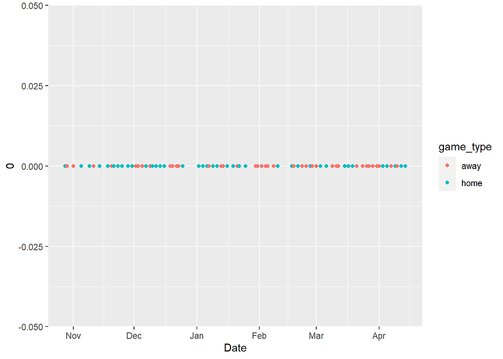
lakers %>%
  ggplot(aes(x = wday(Date, label = TRUE, abbr = FALSE))) +
  geom_bar()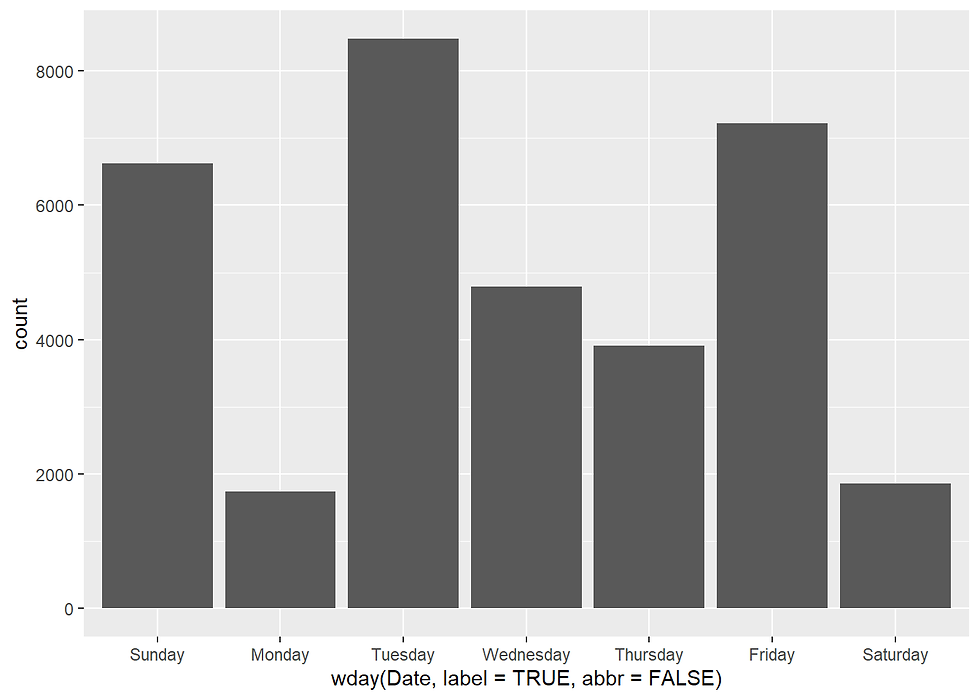
The frequency of basketball games varies throughout the week. Surprisingly, the highest number of games was observed on Tuesdays. The number of games on Saturday is less than 2000.
To look at the distribution of plays throughout the game. The lakers data set lists the time that appeared on the game clock for each play. These times begin at 12:00 at the beginning of each period and then count down to 00:00, which marks the end of the period. The first two digits refer to the number of minutes left in the period. The second two digits refer to the number of seconds.
The times have not been parsed as date-time data to R. It would be difficult to record the time data as a date-time object because the data is incomplete: a minutes and seconds element are not sufficient to identify a unique instant of time. However, we can store the minutes and seconds information as a period object, using the ms() parse function.
lakers$time <- ms(lakers$time)Since periods have relative lengths, it is dangerous to compare them to each other. So we should next convert our periods to durations, which have exact lengths.
lakers$time <- as.duration(lakers$time)This allows us to directly compare different durations. It would also allow us to determine exactly when each play occurred by adding the duration to the instant the game began. (Unfortunately, the starting time for each game is not available in the data set). However, we can still calculate when in each game each play occurred. Each period of play is 12 minutes long and overtime—the 5th period—is 5 minutes long. At the start of each period, the game clock begins counting down from 12:00. So to calculate how much play time elapses before each play, we subtract the time that appears on the game clock from a duration of 12, 24, 36, 48, or 53 minutes (depending on the period of play). We now have a new duration that shows exactly how far into the game each play occurred.
lakers$time <- dminutes(c(12, 24, 36, 48, 53)[lakers$period]) - lakers$timeWe can now plot the number of events over time within each game. We can plot the time of each event as a duration, which will display the number of seconds into the game each play occurred on the x axis,
qplot(time, data = lakers, geom = "histogram", binwidth = 60)
We can also take advantage of pretty.date() to make pretty tick marks by first transforming each duration into a date-time. This helper function recognizes the most intuitive binning and labeling of date-time data, which further enhances our graph. To change durations into datetimes we can just add them all to the same date-time. It does not matter which date we chose. Since the range of our data occurs entirely within an hour, only the minutes information will display in the graph.
lakers$minutes <- ymd("2008-01-01") + lakers$time qplot(minutes, data = lakers, geom = "histogram", binwidth = 60)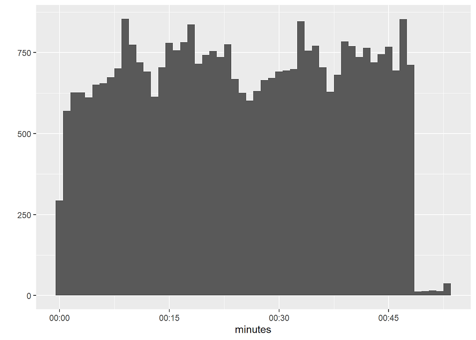
We see that the number of plays peaks within each of the four periods and then plummets at the beginning of the next period. The most plays occur in the last minute of the game. Perhaps any shot is worth taking at this point or there’s less of an incentive not to foul other players. Fewer plays occur in overtime, since not all games go to overtime. Now lets look more closely at just one basketball game: the game played against the Boston Celtics on Christmas of 2008. We can quickly model the amounts of time that occurred between each shot attempt.
game1 <- lakers[lakers$date == "20081225",]
attempts <- game1[game1$etype == "shot",]
The waiting times between shots will be the timespan that occurs between each shot attempt. Since we have recorded the time of each shot attempt as a duration (above), we can record the differences by subtracting the two durations. This automatically creates a new duration whose length is equal to the difference between the first two durations.
attempts$wait <- c(attempts$time[1],  diff(attempts$time))
qplot(as.integer(wait), data = attempts,
                                geom = "histogram",
                                binwidth = 2)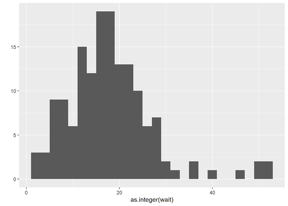
library(plyr)
game1_scores  <- ddply(game1, "team", transform, score = cumsum(points))
game1_scores <- game1_scores[game1_scores$team != "OFF",]
qplot(ymd("2008-01-01") + time, score, data = game1_scores,geom = "line", colour = team)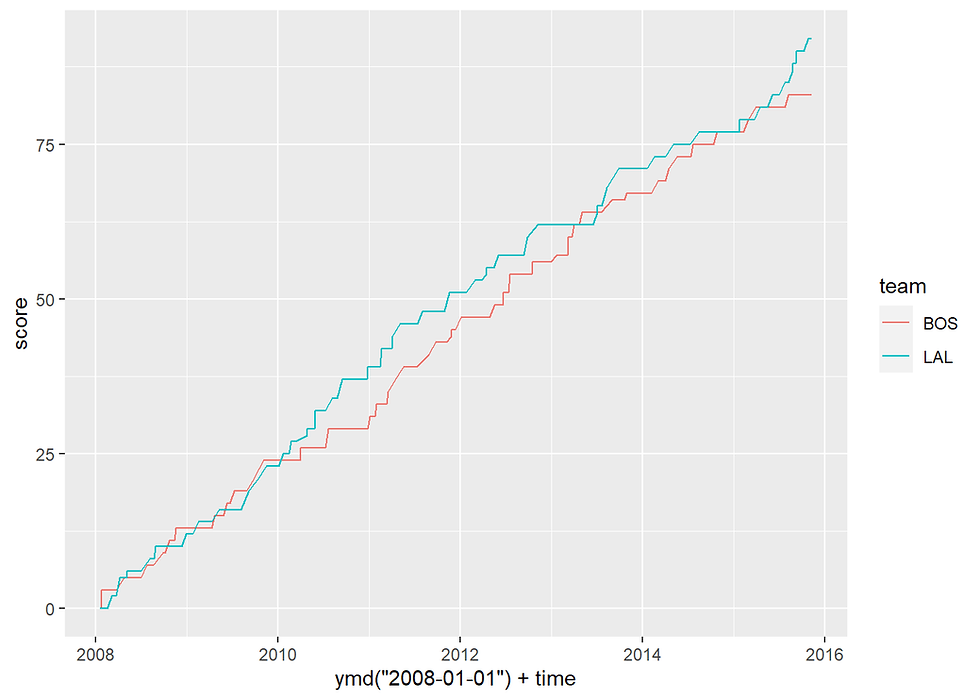

Comments