


Queries using Apache Hive and R codes
- sam33frodon
- Jan 11, 2021
- 4 min read
Updated: Jan 25, 2021
This post presents the R code and Hive code to achieve the same result.
The data set used are station and trip (SF Bay Area Bike Share).
library(tidyverse)
library(dplyr)
library(readr)
To read the two files, we can use read_csv.
station <- read_csv("station_data.csv", col_names = FALSE)## Parsed with column specification:
## cols(
## X1 = col_double(),
## X2 = col_character(),
## X3 = col_double(),
## X4 = col_double(),
## X5 = col_double(),
## X6 = col_character(),
## X7 = col_character()
## )trip <- read_csv("trip_data.csv", col_names = FALSE)## Parsed with column specification:
## cols(
## X1 = col_double(),
## X2 = col_double(),
## X3 = col_character(),
## X4 = col_character(),
## X5 = col_double(),
## X6 = col_character(),
## X7 = col_character(),
## X8 = col_double(),
## X9 = col_double(),
## X10 = col_character(),
## X11 = col_character()
## )Column names are not available. Therefore, we can assign the column names as folliow:
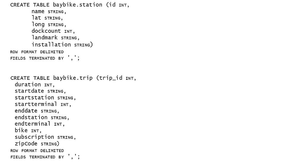
colnames(station) <- c("id","Name","lat","long","dockcount","landmark","installation")

colnames(trip) <- c("trip_id","duration","startdate","startstation","startterminal", "enddate","endstation","endterminal","bike", "subscriptionType", "ZzipCode")
We can have a first look at the two tables
head(trip)## # A tibble: 6 x 11
## trip_id duration startdate startstation startterminal enddate endstation
## <dbl> <dbl> <chr> <chr> <dbl> <chr> <chr>
## 1 913460 765 8/31/201~ Harry Bridg~ 50 8/31/2~ San Franc~
## 2 913459 1036 8/31/201~ San Antonio~ 31 8/31/2~ Mountain ~
## 3 913455 307 8/31/201~ Post at Kea~ 47 8/31/2~ 2nd at So~
## 4 913454 409 8/31/201~ San Jose Ci~ 10 8/31/2~ San Salva~
## 5 913453 789 8/31/201~ Embarcadero~ 51 8/31/2~ Embarcade~
## 6 913452 293 8/31/201~ Yerba Buena~ 68 8/31/2~ San Franc~
## # ... with 4 more variables: endterminal <dbl>, bike <dbl>,
## # subscriptionType <chr>, ZzipCode <chr>head(station)## # A tibble: 6 x 7
## id Name lat long dockcount landmark installation
## <dbl> <chr> <dbl> <dbl> <dbl> <chr> <chr>
## 1 2 San Jose Diridon Caltrain S~ 37.3 -122. 27 San Jose 8/6/2013
## 2 3 San Jose Civic Center 37.3 -122. 15 San Jose 8/5/2013
## 3 4 Santa Clara at Almaden 37.3 -122. 11 San Jose 8/6/2013
## 4 5 Adobe on Almaden 37.3 -122. 19 San Jose 8/5/2013
## 5 6 San Pedro Square 37.3 -122. 15 San Jose 8/7/2013
## 6 7 Paseo de San Antonio 37.3 -122. 15 San Jose 8/7/2013In Apache Hive, we can create tables with the column names:
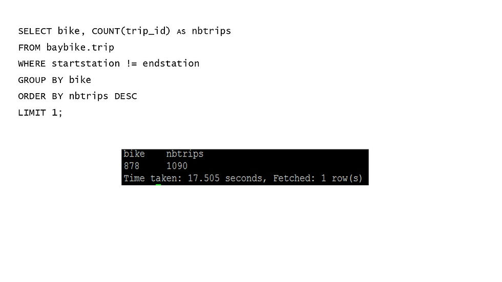
We would like to find the most popular bike, i.e. the bike that has made the highest number of trips (Exclude trips that start and end at the same station).We can use the following R code:
trip %>%
  filter(!startterminal == endterminal) %>%
  group_by(bike) %>%
  count(sort=TRUE) %>%
  head(1)
## # A tibble: 1 x 2
## # Groups: bike [1]
## bike n
## <dbl> <int>
## 1 878 1090So, the bike which is the most used is 878, with 1090 trips. The following Hive code gives the same result
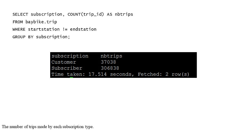
There are two kinds of subscription: customer and subscriber. We can find the number of trips made by each subscription type
trip %>%
  filter(!startterminal == endterminal) %>%
  group_by(subscriptionType) %>%
  count()
## # A tibble: 2 x 2
## # Groups: subscriptionType [2]
## subscriptionType n
## <chr> <int>
## 1 Customer 37038
## 2 Subscriber 306838Clearly, subscriber type made more trips than customer type.
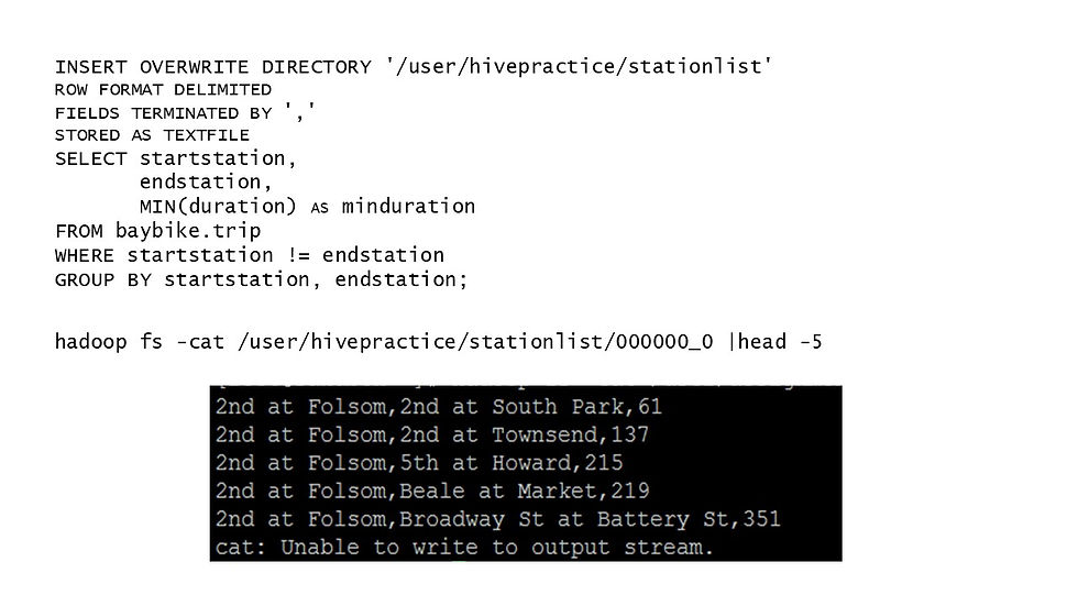
Now, if we want to know the minimum of duration between two stations (Assuming that we do not know the map of BF share bike), we can create a table presenting the two stations and the minimum duration between them.
Here is the R code to see the first 5 rows of the table.
trip %>%
  filter(!startstation == endstation) %>%
  group_by(startstation, endstation) %>%
  summarise(minduration=min(duration)) %>%
  arrange(startstation,endstation, minduration) %>%
  head(5)
## # A tibble: 5 x 3
## # Groups: startstation [1]
## startstation endstation minduration
## <chr> <chr> <dbl>
## 1 2nd at Folsom 2nd at South Park 61
## 2 2nd at Folsom 2nd at Townsend 137
## 3 2nd at Folsom 5th at Howard 215
## 4 2nd at Folsom Beale at Market 219
## 5 2nd at Folsom Broadway St at Battery St 351
The Hive code also gives the same output
If we want to know the number of trips originating from each landmark, we need to join the two tables.
table1 <- trip %>%
  left_join(station, by = c("startterminal" = "id"))

table2 <- table1 %>%
  filter(!startstation == endstation) %>%
  group_by(landmark) %>%
  count()
## # A tibble: 5 x 2
## # Groups: landmark [5]
## landmark n
## <chr> <int>
## 1 Mountain View 9361
## 2 Palo Alto 2370
## 3 Redwood City 1790
## 4 San Francisco 313528
## 5 San Jose 16827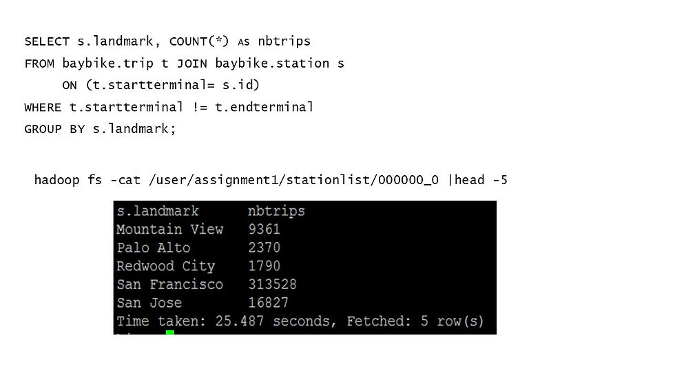
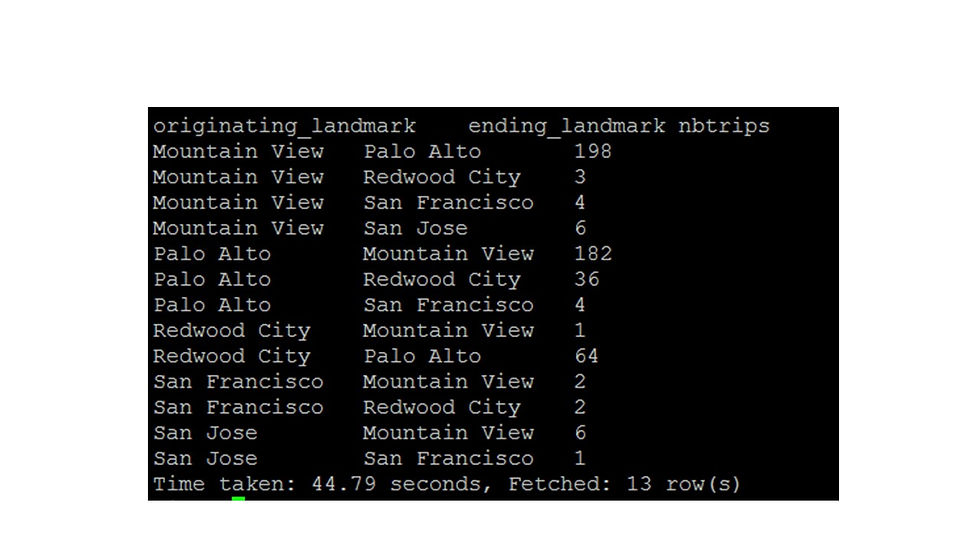
Finally, we can create a table showing number of trips crossing landmarks, i.e trips that originate in one landmark and end in another.
table3 <- trip %>%
  left_join(station, by = c("startterminal" = "id"))

colnames(table3)[colnames(table3)=="landmark"] <- "start_landmark"

table4 <- trip %>%
  left_join(station, by =  c("endterminal"= "id"))

colnames(table4)[colnames(table4)=="landmark"] <- "end_landmark"

table3 %>%
  left_join(table4, by = c("trip_id" = "trip_id"))%>%
  filter(!start_landmark == end_landmark) %>%
  group_by(start_landmark, end_landmark) %>%
  count()
## # A tibble: 13 x 3
## # Groups: start_landmark, end_landmark [13]
## start_landmark end_landmark n
## <chr> <chr> <int>
## 1 Mountain View Palo Alto 198
## 2 Mountain View Redwood City 3
## 3 Mountain View San Francisco 4
## 4 Mountain View San Jose 6
## 5 Palo Alto Mountain View 182
## 6 Palo Alto Redwood City 36
## 7 Palo Alto San Francisco 4
## 8 Redwood City Mountain View 1
## 9 Redwood City Palo Alto 64
## 10 San Francisco Mountain View 2
## 11 San Francisco Redwood City 2
## 12 San Jose Mountain View 6
## 13 San Jose San Francisco 1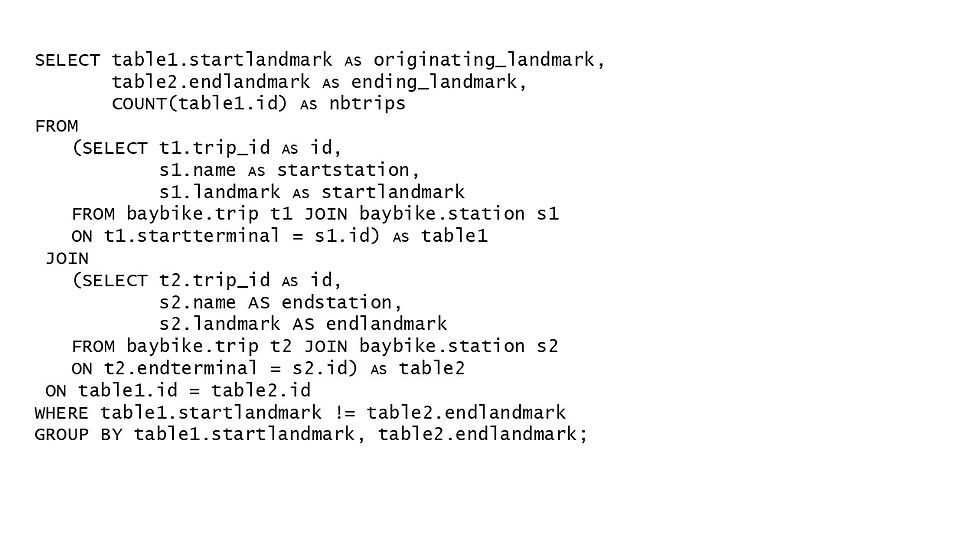
Comments