


RFM score as input for K-means clustering
- sam33frodon
- Dec 28, 2020
- 7 min read
Updated: Jan 12, 2021
An RFM (recency, frequency, and monetary value) analysis tells you which customers are likely to respond to a new offer.
The RFM analysis assigns a 3 digit RFM score (from 111 thru 555) to each customer. A score of 555 indicates that a customer has purchased a product or service most recently, most frequently, and at the highest monetary value.
Reading data from csv file
library(readr)
data <- read_csv("customerFMCG.csv")
## Parsed with column specification:
## cols(
## Invoice_No = col_double(),
## Stock_Code = col_double(),
## Product_Category = col_character(),
## Invoice_Date = col_character(),
## Customer_ID = col_double(),
## Amount = col_double(),
## Country = col_character(),
## l_Date = col_character()
## )str(data)## Classes 'spec_tbl_df', 'tbl_df', 'tbl' and 'data.frame': 330379 obs. of 8 variables:
## $ Invoice_No : num 1540425 1540425 1540425 1540425 1540425 ...
## $ Stock_Code : num 154735 154063 153547 153547 153547 ...
## $ Product_Category: chr "Healthcare & Beauty" "Toiletries" "Grocery" "Grocery" ...
## $ Invoice_Date : chr "1/7/2011" "1/7/2011" "1/7/2011" "1/7/2011" ...
## $ Customer_ID : num 556591 556591 556591 556591 556591 ...
## $ Amount : num 23.4 13.6 14.6 13.6 14.8 ...
## $ Country : chr "United States" "United States" "United States" "United States" ...
## $ l_Date : chr "12/12/2011" "12/12/2011" "12/12/2011" "12/12/2011" ...
## - attr(*, "spec")=
## .. cols(
## .. Invoice_No = col_double(),
## .. Stock_Code = col_double(),
## .. Product_Category = col_character(),
## .. Invoice_Date = col_character(),
## .. Customer_ID = col_double(),
## .. Amount = col_double(),
## .. Country = col_character(),
## .. l_Date = col_character()
## .. )2. Data description
Invoice_No (Numeric): Invoice no for each transaction
Stock_Code (Numeric): Unique stock code for the items
Product_Category (Categorical): Product category details
Invoice_Date (Numeric): Date on which invoice was generated
Customer_ID (Numeric): Unique customer id
Amount (Numeric): Invoice Amount
Country(Categorical): Country
detail l_date(Numeric): Last date of invoice in 2011
library(DataExplorer)3. Data profiling
Checking if there are missing values
plot_missing(data)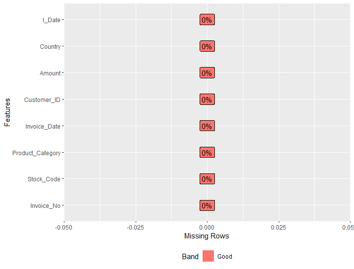
Examine the first 10 rows of the data
head(data,10)## # A tibble: 10 x 8
## Invoice_No Stock_Code Product_Category Invoice_Date Customer_ID Amount
## <dbl> <dbl> <chr> <chr> <dbl> <dbl>
## 1 1540425 154735 Healthcare & Be~ 1/7/2011 556591 23.4
## 2 1540425 154063 Toiletries 1/7/2011 556591 13.6
## 3 1540425 153547 Grocery 1/7/2011 556591 14.6
## 4 1540425 153547 Grocery 1/7/2011 556591 13.6
## 5 1540425 153547 Grocery 1/7/2011 556591 14.8
## 6 1540425 154735 Healthcare & Be~ 1/7/2011 556591 23.4
## 7 1540425 153547 Grocery 1/7/2011 556591 24.4
## 8 1540425 154735 Healthcare & Be~ 1/7/2011 556591 22.1
## 9 1540425 153547 Grocery 1/7/2011 556591 20.5
## 10 1540425 217510 Beverages 1/7/2011 556591 19.2
## # ... with 2 more variables: Country <chr>, l_Date <chr>str(data)## Classes 'spec_tbl_df', 'tbl_df', 'tbl' and 'data.frame': 330379 obs. of 8 variables:
## $ Invoice_No : num 1540425 1540425 1540425 1540425 1540425 ...
## $ Stock_Code : num 154735 154063 153547 153547 153547 ...
## $ Product_Category: chr "Healthcare & Beauty" "Toiletries" "Grocery" "Grocery" ...
## $ Invoice_Date : chr "1/7/2011" "1/7/2011" "1/7/2011" "1/7/2011" ...
## $ Customer_ID : num 556591 556591 556591 556591 556591 ...
## $ Amount : num 23.4 13.6 14.6 13.6 14.8 ...
## $ Country : chr "United States" "United States" "United States" "United States" ...
## $ l_Date : chr "12/12/2011" "12/12/2011" "12/12/2011" "12/12/2011" ...
## - attr(*, "spec")=
## .. cols(
## .. Invoice_No = col_double(),
## .. Stock_Code = col_double(),
## .. Product_Category = col_character(),
## .. Invoice_Date = col_character(),
## .. Customer_ID = col_double(),
## .. Amount = col_double(),
## .. Country = col_character(),
## .. l_Date = col_character()
## .. )library(dplyr)Counting unique values
n_distinct(data$Invoice_No) ## [1] 15355n_distinct(data$Stock_Code) ## [1] 5data %>%
group_by(Product_Category) %>%
count()## # A tibble: 5 x 2
## # Groups: Product_Category [5]
## Product_Category n
## <chr> <int>
## 1 Beverages 35382
## 2 Dairy 41412
## 3 Grocery 204526
## 4 Healthcare & Beauty 40209
## 5 Toiletries 8850library(pander)
library(ggplot2)
library(scales)df_category <- data %>%
group_by(Product_Category) %>%
summarise(Count = n()) %>%
arrange(-Count) %>%
mutate(Percentage = round(Count*100/sum(Count),2),
label = percent(Percentage/100))
df_category## # A tibble: 5 x 4
## Product_Category Count Percentage label
## <chr> <int> <dbl> <chr>
## 1 Grocery 204526 61.9 61.91%
## 2 Dairy 41412 12.5 12.53%
## 3 Healthcare & Beauty 40209 12.2 12.17%
## 4 Beverages 35382 10.7 10.71%
## 5 Toiletries 8850 2.68 2.68%ggplot(df_category,
aes(x = reorder(Product_Category, -Percentage),
y = Percentage)) +
geom_bar(stat = "identity",
fill = "royalblue4",
width = 0.80) +
geom_text(aes(label = paste0(Percentage,"%")),
vjust = -0.3,
size = 4,
fontface = "bold") +
labs(x = "Category",
y = "Distribution of product category (%)") +
theme(axis.text = element_text(size = 12),
axis.title = element_text(size = 12, face = "bold"),
plot.caption = element_text(color = "grey44",size = 12,face = "italic"),
legend.text = element_text(colour="black", size = 12))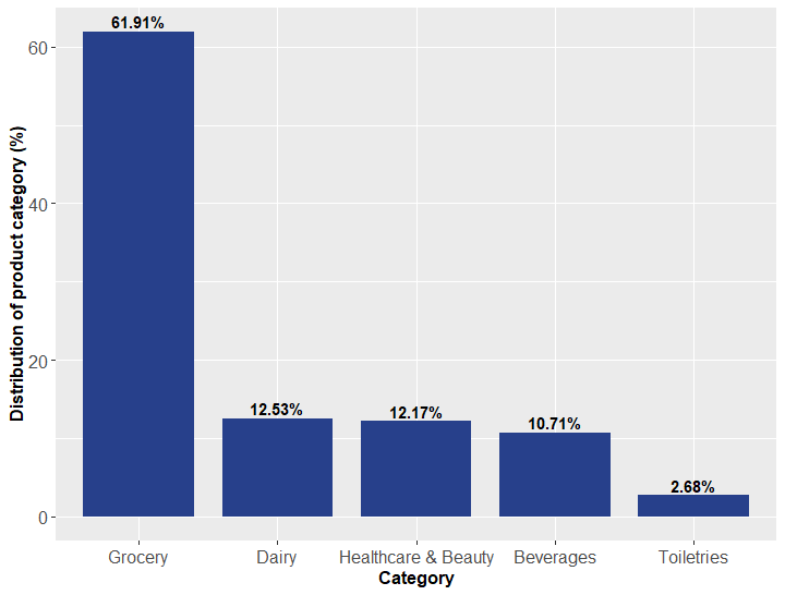
n_distinct(data$Customer_ID)## [1] 3813There are 3813 unique customers and 15335 unique invoice numbers.
Formatting Date
head(data$l_Date)## [1] "12/12/2011" "12/12/2011" "12/12/2011" "12/12/2011" "12/12/2011"
## [6] "12/12/2011"data2 <- data %>%
mutate(Invoice_Date = as.Date(Invoice_Date, "%m/%d/%Y"))str(data2)## Classes 'spec_tbl_df', 'tbl_df', 'tbl' and 'data.frame': 330379 obs. of 8 variables:
## $ Invoice_No : num 1540425 1540425 1540425 1540425 1540425 ...
## $ Stock_Code : num 154735 154063 153547 153547 153547 ...
## $ Product_Category: chr "Healthcare & Beauty" "Toiletries" "Grocery" "Grocery" ...
## $ Invoice_Date : Date, format: "2011-01-07" "2011-01-07" ...
## $ Customer_ID : num 556591 556591 556591 556591 556591 ...
## $ Amount : num 23.4 13.6 14.6 13.6 14.8 ...
## $ Country : chr "United States" "United States" "United States" "United States" ...
## $ l_Date : chr "12/12/2011" "12/12/2011" "12/12/2011" "12/12/2011" ...data2 %>%
group_by(Country) %>%
count()## # A tibble: 1 x 2
## # Groups: Country [1]
## Country n
## <chr> <int>
## 1 United States 330379All these records belong to only one country. We will not need this column.
summary(data2$Amount)## Min. 1st Qu. Median Mean 3rd Qu. Max.
## 1.00 6.57 13.65 24.67 22.14 185319.56hist(data2$Amount)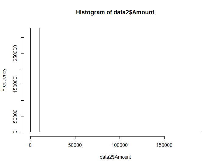
 ggplot(data2, aes(x = "", y = Amount)) +
  geom_boxplot()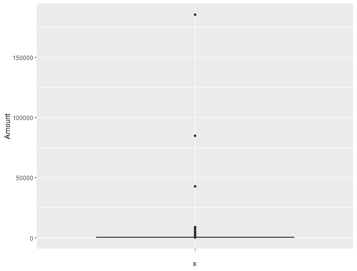
There are outliers.
data2 %>%
  group_by(l_Date) %>%
  count()
## # A tibble: 1 x 2
## # Groups: l_Date [1]
## l_Date n
## <chr> <int>
## 1 12/12/2011 330379This column is redundant.
4. Building RFM model
R_table <- aggregate(Invoice_Date ~ Customer_ID, data2, FUN = max)data2 %>%
group_by(Customer_ID) %>%
summarise(max = max(Invoice_Date))## # A tibble: 3,813 x 2
## Customer_ID max
## <dbl> <date>
## 1 555624 2011-01-21
## 2 556025 2011-12-10
## 3 556026 2011-12-12
## 4 556027 2011-12-09
## 5 556098 2011-12-09
## 6 556099 2011-05-12
## 7 556100 2011-10-03
## 8 556101 2011-09-29
## 9 556102 2011-10-14
## 10 556104 2011-12-10
## # ... with 3,803 more rowshead(R_table)## Customer_ID Invoice_Date
## 1 555624 2011-01-21
## 2 556025 2011-12-10
## 3 556026 2011-12-12
## 4 556027 2011-12-09
## 5 556098 2011-12-09
## 6 556099 2011-05-12NOW <- as.Date("2011-12-12", "%Y-%m-%d")
NOW## [1] "2011-12-12"R_table$R <- as.numeric(NOW - R_table$Invoice_Date)head(R_table)## Customer_ID Invoice_Date R
## 1 555624 2011-01-21 325
## 2 556025 2011-12-10 2
## 3 556026 2011-12-12 0
## 4 556027 2011-12-09 3
## 5 556098 2011-12-09 3
## 6 556099 2011-05-12 214RFM_data <- data2 %>%
group_by(Customer_ID) %>%
summarise(Recency = as.numeric(NOW - max(Invoice_Date)),
Frequency = length(Invoice_Date),
Monetary = sum(Amount)) str(RFM_data)## Classes 'tbl_df', 'tbl' and 'data.frame': 3813 obs. of 4 variables:
## $ Customer_ID: num 555624 556025 556026 556027 556098 ...
## $ Recency : num 325 2 0 3 3 214 70 74 59 2 ...
## $ Frequency : int 1 88 3927 199 59 6 46 5 25 82 ...
## $ Monetary : num 84903 4015 40338 4903 1147 ...head(RFM_data)## # A tibble: 6 x 4
## Customer_ID Recency Frequency Monetary
## <dbl> <dbl> <int> <dbl>
## 1 555624 325 1 84903.
## 2 556025 2 88 4015.
## 3 556026 0 3927 40338.
## 4 556027 3 199 4903.
## 5 556098 3 59 1147.
## 6 556099 214 6 116.RFM scoring
Rsegment 1 is very recent while Rsegment 5 is least recent. In this step, scoring the RFM data is done by using the quantile method. The scoring is in a range of 1 to 5.
Rsegment 1 is very recent while Rsegment 5 is the least recent score.
Fsegment 1 is least frequent while Fsegment 5 is most frequent
RFM_data <- RFM_data %>%
  mutate(Rsegment = findInterval(Recency, quantile(Recency, c(0.0, 0.25, 0.50, 0.75, 1.0))),
         Fsegment = findInterval(Frequency, quantile(Frequency, c(0.0, 0.25, 0.50, 0.75, 1.0))),
         Msegment = findInterval(Monetary, quantile(Monetary, c(0.0, 0.25, 0.50, 0.75, 1.0))),
         R_F_M = paste(Rsegment, Fsegment, Msegment),
Total_RFM_Score = c(Rsegment + Fsegment + Msegment))head(RFM_data)## # A tibble: 6 x 9
## Customer_ID Recency Frequency Monetary Rsegment Fsegment Msegment R_F_M
## <dbl> <dbl> <int> <dbl> <int> <int> <int> <chr>
## 1 555624 325 1 84903. 4 1 4 4 1 4
## 2 556025 2 88 4015. 1 3 4 1 3 4
## 3 556026 0 3927 40338. 1 4 4 1 4 4
## 4 556027 3 199 4903. 1 4 4 1 4 4
## 5 556098 3 59 1147. 1 3 3 1 3 3
## 6 556099 214 6 116. 4 1 1 4 1 1
## # ... with 1 more variable: Total_RFM_Score <int>To keep only selected variables from RFM data
clus_df2 <- RFM_data[,c(5,6,7)]Applying K-means
set.seed(123)
km2 <- kmeans(clus_df2, centers = 5, nstart = 30)
str(km2) ## List of 9
## $ cluster : int [1:3813] 5 2 2 2 2 3 4 5 5 2 ...
## $ centers : num [1:5, 1:3] 1.63 1 3.66 2.48 3.56 ...
## ..- attr(*, "dimnames")=List of 2
## .. ..$ : chr [1:5] "1" "2" "3" "4" ...
## .. ..$ : chr [1:3] "Rsegment" "Fsegment" "Msegment"
## $ totss : num 14187
## $ withinss : num [1:5] 872 352 417 864 668
## $ tot.withinss: num 3174
## $ betweenss : num 11013
## $ size : int [1:5] 700 679 789 931 714
## $ iter : int 3
## $ ifault : int 0
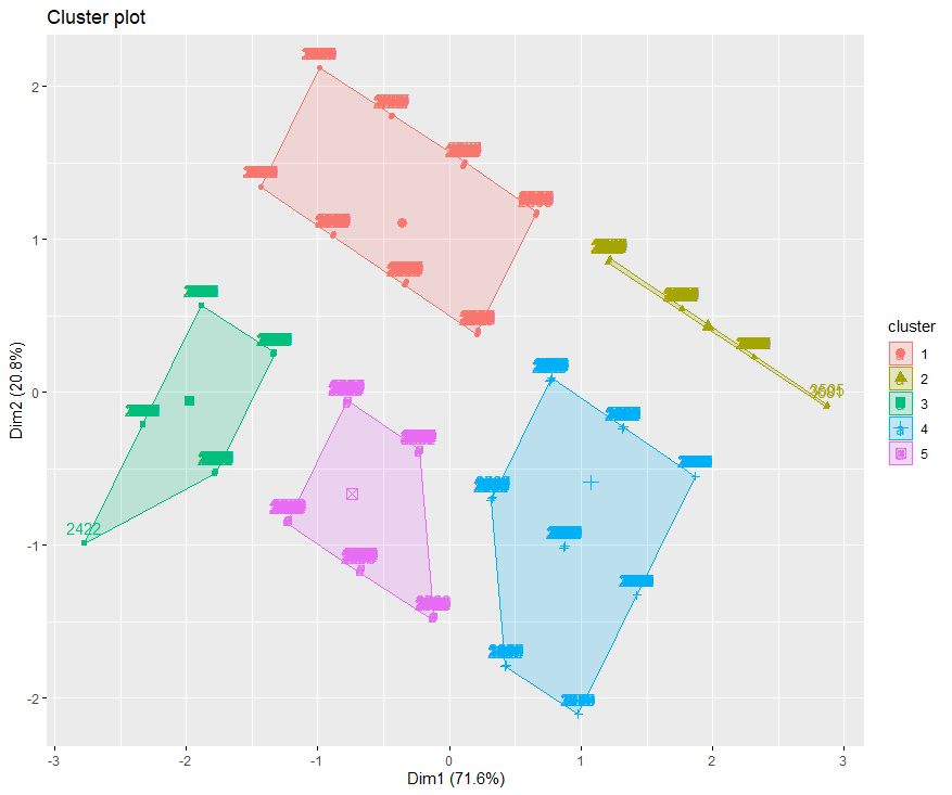
## - attr(*, "class")= chr "kmeans"library(factoextra)fviz_cluster(km2, data = clus_df2)finalclus2 <- cbind(clus_df2,km2$cluster)finalclus2 %>%
group_by(km2$cluster) %>%
count()## # A tibble: 5 x 2
## # Groups: km2$cluster [5]
## `km2$cluster` n
## <int> <int>
## 1 1 700
## 2 2 679
## 3 3 789
## 4 4 931
## 5 5 714
Comments