Dealing with missing data : Mean imputation (Using R)

library(tidyverse)

library(DataExplorer)
library(dplyr)

A. Detecting missing values

data <- read.csv(file = "https://raw.githubusercontent.com/agconti/kaggle-titanic/master/data/train.csv", header = T, sep = ",")

str(data)

## 'data.frame':    891 obs. of  12 variables:
##  $ PassengerId: int  1 2 3 4 5 6 7 8 9 10 ...
##  $ Survived   : int  0 1 1 1 0 0 0 0 1 1 ...
##  $ Pclass     : int  3 1 3 1 3 3 1 3 3 2 ...
##  $ Name       : Factor w/ 891 levels "Abbing, Mr. Anthony",..: 109 191 358 277 16 559 520 629 417 581 ...
##  $ Sex        : Factor w/ 2 levels "female","male": 2 1 1 1 2 2 2 2 1 1 ...
##  $ Age        : num  22 38 26 35 35 NA 54 2 27 14 ...
##  $ SibSp      : int  1 1 0 1 0 0 0 3 0 1 ...
##  $ Parch      : int  0 0 0 0 0 0 0 1 2 0 ...
##  $ Ticket     : Factor w/ 681 levels "110152","110413",..: 524 597 670 50 473 276 86 396 345 133 ...
##  $ Fare       : num  7.25 71.28 7.92 53.1 8.05 ...
##  $ Cabin      : Factor w/ 148 levels "","A10","A14",..: 1 83 1 57 1 1 131 1 1 1 ...
##  $ Embarked   : Factor w/ 4 levels "","C","Q","S": 4 2 4 4 4 3 4 4 4 2 ...

The data contain 891 observations and 12 variables.

Interger and numeric type : PassengerId, Survived, Pclass, Age, SibSp, Parch.

Fare Factor type: Name, Sex, Ticket, Cabin, Embarked.

Description of the data set

PassengerID: Id of passengers Survived: (0 = No; 1 = Yes)

Pclass: Passenger Class (1 = 1st; 2 = 2nd; 3 = 3rd)

Name: Name

Sex: Genders of passengers

Age: Age

Sibsp: Number of Siblings/Spouses

Aboard Parch: Number of Parents/Children Aboard

Ticket: Ticket Number

Fare: Passenger Fare (British pound)

Cabin: Cabin Embarked: Port of Embarkation (C = Cherbourg; Q = Queenstown; S = Southampton)

We can also plot the summary above using plot_intro function.

plot_intro(data)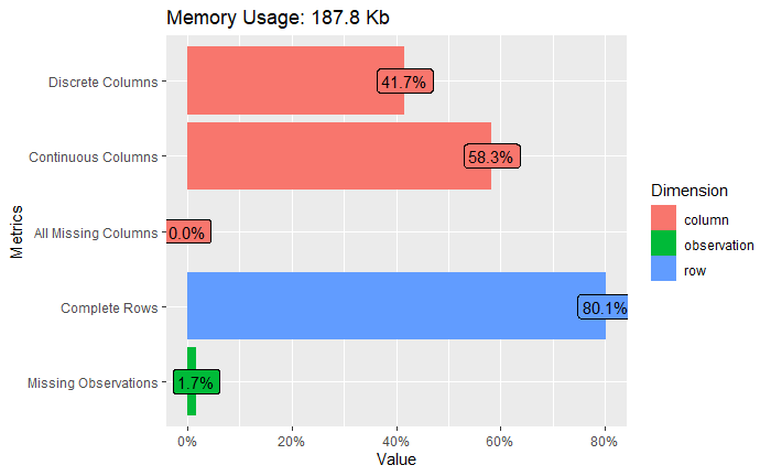

There are 5 discrete columns and 7 continuous columns, corresponding to the 5 columns of factor type and to the 7 columns of numeric and integer type, respectively.

There are 177 missing values and 714 completed rows.

There are 10692 observations = 891 rows * 12 variables = 10692 There is 1.7% missing observations (177/10692 = 1.655%) complete rows :80.1% (714/891 = 80.13 %)

If we want to know which column containing missing values

plot_missing(data)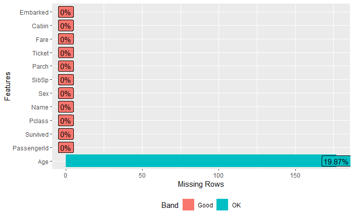

All the missing values are found in the column age. In fact, 19.87 % of data in this column is missing. There are 892 rows. There are 19.87% * 891 = 177 missing rows, in agreement with the summary above.

Other way to check that number

sum(is.na(data$Age))

## [1] 177

If we want to see missing values for each column

sapply(data,function(x)sum(is.na(x)))

## PassengerId    Survived      Pclass        Name         Sex         Age 
##           0           0           0           0           0         177 
##       SibSp       Parch      Ticket        Fare       Cabin    Embarked 
##           0           0           0           0           0           0

data %>%
  sapply(function(x) sum(is.na(x)))

## PassengerId    Survived      Pclass        Name         Sex      Age 
##           0           0           0           0           0      177 
##       SibSp       Parch      Ticket        Fare       Cabin Embarked 
##           0           0           0           0           0        0

B. Imputation using mean

One way to deal with missing values is to replace NA rows by the mean value of the column. In this data set, we only have missing values for the age column. One way to deal with this situation is to replace the missing value by the average age. As the title may be related to the age, we will calculate the average age for each group of people who have the same title. As we have many titles (Mr, Ms, etc…) = many genders, we would assign the average age in function of title. We should know how many titles in this data set what are theses titles ? what are the average age of each of these groups ?

First, we will create a new column that contains only the title. Adding a column title into a data set

How does the name column look like ?

data %>% 
  select(Name) %>% 
  head(10)

##                                                   Name
## 1                              Braund, Mr. Owen Harris
## 2  Cumings, Mrs. John Bradley (Florence Briggs Thayer)
## 3                               Heikkinen, Miss. Laina
## 4         Futrelle, Mrs. Jacques Heath (Lily May Peel)
## 5                             Allen, Mr. William Henry
## 6                                     Moran, Mr. James
## 7                              McCarthy, Mr. Timothy J
## 8                       Palsson, Master. Gosta Leonard
## 9    Johnson, Mrs. Oscar W (Elisabeth Vilhelmina Berg)
## 10                 Nasser, Mrs. Nicholas (Adele Achem)

You can see that the title is included in the name. We should remove the title and create a new column containing only the title

data <- data %>% 
  mutate(Title = regmatches(Name, regexpr("[A-z]+\\.", Name)))

data %>% 
  select(Name, Title) %>% 
  head(10)

##                                                   Name   Title
## 1                              Braund, Mr. Owen Harris     Mr.
## 2  Cumings, Mrs. John Bradley (Florence Briggs Thayer)    Mrs.
## 3                               Heikkinen, Miss. Laina   Miss.
## 4         Futrelle, Mrs. Jacques Heath (Lily May Peel)    Mrs.
## 5                             Allen, Mr. William Henry     Mr.
## 6                                     Moran, Mr. James     Mr.
## 7                              McCarthy, Mr. Timothy J     Mr.
## 8                       Palsson, Master. Gosta Leonard Master.
## 9    Johnson, Mrs. Oscar W (Elisabeth Vilhelmina Berg)    Mrs.
## 10                 Nasser, Mrs. Nicholas (Adele Achem)    Mrs.

To remove titles in the column name

data <- data %>%
  mutate(Name = gsub("[A-z]+\\.","",Name))

To check if titles were removed

data %>% 
  select(Name, Title) %>% 
  head(10)

##                                               Name   Title
## 1                             Braund,  Owen Harris     Mr.
## 2  Cumings,  John Bradley (Florence Briggs Thayer)    Mrs.
## 3                                Heikkinen,  Laina   Miss.
## 4         Futrelle,  Jacques Heath (Lily May Peel)    Mrs.
## 5                            Allen,  William Henry     Mr.
## 6                                    Moran,  James     Mr.
## 7                             McCarthy,  Timothy J     Mr.
## 8                          Palsson,  Gosta Leonard Master.
## 9    Johnson,  Oscar W (Elisabeth Vilhelmina Berg)    Mrs.
## 10                 Nasser,  Nicholas (Adele Achem)    Mrs.

Now, we place the column title in after the column name

data <- data %>% 
  select(PassengerId, Name, Title, Sex, Age, everything())

head(data, 10)

##    PassengerId                                            Name   Title    Sex
## 1            1                            Braund,  Owen Harris     Mr.   male
## 2            2 Cumings,  John Bradley (Florence Briggs Thayer)    Mrs. female
## 3            3                               Heikkinen,  Laina   Miss. female
## 4            4        Futrelle,  Jacques Heath (Lily May Peel)    Mrs. female
## 5            5                           Allen,  William Henry     Mr.   male
## 6            6                                   Moran,  James     Mr.   male
## 7            7                            McCarthy,  Timothy J     Mr.   male
## 8            8                         Palsson,  Gosta Leonard Master.   male
## 9            9   Johnson,  Oscar W (Elisabeth Vilhelmina Berg)    Mrs. female
## 10          10                 Nasser,  Nicholas (Adele Achem)    Mrs. female
##    Age Survived Pclass SibSp Parch           Ticket    Fare Cabin Embarked
## 1   22        0      3     1     0        A/5 21171  7.2500              S
## 2   38        1      1     1     0         PC 17599 71.2833   C85        C
## 3   26        1      3     0     0 STON/O2. 3101282  7.9250              S
## 4   35        1      1     1     0           113803 53.1000  C123        S
## 5   35        0      3     0     0           373450  8.0500              S
## 6   NA        0      3     0     0           330877  8.4583              Q
## 7   54        0      1     0     0            17463 51.8625   E46        S
## 8    2        0      3     3     1           349909 21.0750              S
## 9   27        1      3     0     2           347742 11.1333              S
## 10  14        1      2     1     0           237736 30.0708              C

Counting the title and order the output

data %>% 
group_by (Title) %>%
count(sort = TRUE)

## # A tibble: 17 x 2
## # Groups:   Title [17]
##    Title         n
##    <chr>     <int>
##  1 Mr.         517
##  2 Miss.       182
##  3 Mrs.        125
##  4 Master.      40
##  5 Dr.           7
##  6 Rev.          6
##  7 Col.          2
##  8 Major.        2
##  9 Mlle.         2
## 10 Capt.         1
## 11 Countess.     1
## 12 Don.          1
## 13 Jonkheer.     1
## 14 Lady.         1
## 15 Mme.          1
## 16 Ms.           1
## 17 Sir.          1

There are 17 groups. Mr., Miss., Mrs. are the most common among titles. There are some uncommon titles such as: Capt., Countess., Don., Jonkheer., Lady., Mme., Ms., and Sir.

Checking the number of missing rows by title

data %>%
  group_by(Title) %>% 
  summarise(missing_total = sum(is.na(Age))) %>% 
  arrange(desc(missing_total))

## # A tibble: 17 x 2
##    Title     missing_total
##    <chr>             <int>
##  1 Mr.                 119
##  2 Miss.                36
##  3 Mrs.                 17
##  4 Master.               4
##  5 Dr.                   1
##  6 Capt.                 0
##  7 Col.                  0
##  8 Countess.             0
##  9 Don.                  0
## 10 Jonkheer.             0
## 11 Lady.                 0
## 12 Major.                0
## 13 Mlle.                 0
## 14 Mme.                  0
## 15 Ms.                   0
## 16 Rev.                  0
## 17 Sir.                  0

The missing values were found at corresponding rows : 119 for Mr., 36 for Miss., 17 for Mrs., 4 for Master., and 1 for Dr. Because there are only 5 groups that contain missing values. We will calculate the mean age of these 5 groups rather than 17 groups

data %>%
  filter(Title %in% c("Mr.","Miss.", "Mrs.", "Master.","Dr.")) %>% 
  group_by(Title) %>% 
  summarise (average = mean(Age, na.rm = TRUE))

## # A tibble: 5 x 2
##   Title   average
##   <chr>     <dbl>
## 1 Dr.       42   
## 2 Master.    4.57
## 3 Miss.     21.8 
## 4 Mr.       32.4 
## 5 Mrs.      35.9

Miss., 182 rows, the average age = 21.77 Mr., 517 rows, the average age = 32.36 Mrs.,125 rows, the average age= 35.89 Master., 40 rows, the average age = 4.57

Assign the missing values of the age column by respectable values Now, we can replace missing values by the mean of corresponding groups

data <- data %>% 
  mutate(Age = case_when(Title == "Mr." & is.na(Age) ~ mean(Age[Title == "Mr."], na.rm = TRUE),
                         Title == "Miss." & is.na(Age)~ mean(Age[Title == "Miss."], na.rm = TRUE),
                         Title == "Mrs." & is.na(Age) ~ mean(Age[Title == "Mrs."], na.rm = TRUE),
                         Title == "Master." & is.na(Age) ~ mean(Age[Title == "Master."], na.rm = TRUE), 
                         Title == "Dr." & is.na(Age) ~ mean(Age[Title == "Dr."], na.rm = TRUE),
                         TRUE ~ Age))

sum(is.na(data$Age))

## [1] 0

Other way to replace missing value.

train$Age[train$Title == "Mr." & is.na(train$Age)] <- mean(train$Age[train$Title == "Mr."], na.rm = TRUE)

train$Age[train$Title == "Miss." & is.na(train$Age)] <- mean(train$Age[train$Title == "Miss."], na.rm = TRUE)

train$Age[train$Title == "Mrs." & is.na(train$Age)] <- mean(train$Age[train$Title == "Mrs."], na.rm = TRUE)

train$Age[train$Title == "Master." & is.na(train$Age)] <- mean(train$Age[train$Title == "Master."], na.rm = TRUE)