Tidyverse vs Pandas

1. Reading data

In Tidyverse

library(tidyverse)
df_movies <- read.csv("movies.csv")

In Python

import numpy as np
import pandas as pd
df_movies = pd.read_csv(‘movies.csv’, index_col=‘id’, low_memory=False)

2. To obtain information about columns, datatypes and memory footprint.

In Tidyverse

str(df_movies)

## 'data.frame':    45466 obs. of  24 variables:
##  $ adult                : chr  "False" "False" "False" "False" ...
##  $ belongs_to_collection: chr  "{'id': 10194, 'name': 'Toy Story Collection', 'poster_path': '/7G9915LfUQ2lVfwMEEhDsn3kT4B.jpg', 'backdrop_path"| __truncated__ "" "{'id': 119050, 'name': 'Grumpy Old Men Collection', 'poster_path': '/nLvUdqgPgm3F85NMCii9gVFUcet.jpg', 'backdro"| __truncated__ "" ...
##  $ budget               : chr  "30000000" "65000000" "0" "16000000" ...
##  $ genres               : chr  "[{'id': 16, 'name': 'Animation'}, {'id': 35, 'name': 'Comedy'}, {'id': 10751, 'name': 'Family'}]" "[{'id': 12, 'name': 'Adventure'}, {'id': 14, 'name': 'Fantasy'}, {'id': 10751, 'name': 'Family'}]" "[{'id': 10749, 'name': 'Romance'}, {'id': 35, 'name': 'Comedy'}]" "[{'id': 35, 'name': 'Comedy'}, {'id': 18, 'name': 'Drama'}, {'id': 10749, 'name': 'Romance'}]" ...
##  $ homepage             : chr  "http://toystory.disney.com/toy-story" "" "" "" ...
##  $ id                   : chr  "862" "8844" "15602" "31357" ...
##  $ imdb_id              : chr  "tt0114709" "tt0113497" "tt0113228" "tt0114885" ...
##  $ original_language    : chr  "en" "en" "en" "en" ...
##  $ original_title       : chr  "Toy Story" "Jumanji" "Grumpier Old Men" "Waiting to Exhale" ...
##  $ overview             : chr  "Led by Woody, Andy's toys live happily in his room until Andy's birthday brings Buzz Lightyear onto the scene. "| __truncated__ "When siblings Judy and Peter discover an enchanted board game that opens the door to a magical world, they unwi"| __truncated__ "A family wedding reignites the ancient feud between next-door neighbors and fishing buddies John and Max. Meanw"| __truncated__ "Cheated on, mistreated and stepped on, the women are holding their breath, waiting for the elusive \"good man\""| __truncated__ ...
##  $ popularity           : chr  "21.946943" "17.015539" "11.7129" "3.859495" ...
##  $ poster_path          : chr  "/rhIRbceoE9lR4veEXuwCC2wARtG.jpg" "/vzmL6fP7aPKNKPRTFnZmiUfciyV.jpg" "/6ksm1sjKMFLbO7UY2i6G1ju9SML.jpg" "/16XOMpEaLWkrcPqSQqhTmeJuqQl.jpg" ...
##  $ production_companies : chr  "[{'name': 'Pixar Animation Studios', 'id': 3}]" "[{'name': 'TriStar Pictures', 'id': 559}, {'name': 'Teitler Film', 'id': 2550}, {'name': 'Interscope Communicat"| __truncated__ "[{'name': 'Warner Bros.', 'id': 6194}, {'name': 'Lancaster Gate', 'id': 19464}]" "[{'name': 'Twentieth Century Fox Film Corporation', 'id': 306}]" ...
##  $ production_countries : chr  "[{'iso_3166_1': 'US', 'name': 'United States of America'}]" "[{'iso_3166_1': 'US', 'name': 'United States of America'}]" "[{'iso_3166_1': 'US', 'name': 'United States of America'}]" "[{'iso_3166_1': 'US', 'name': 'United States of America'}]" ...
##  $ release_date         : chr  "1995-10-30" "1995-12-15" "1995-12-22" "1995-12-22" ...
##  $ revenue              : num  3.74e+08 2.63e+08 0.00 8.15e+07 7.66e+07 ...
##  $ runtime              : num  81 104 101 127 106 170 127 97 106 130 ...
##  $ spoken_languages     : chr  "[{'iso_639_1': 'en', 'name': 'English'}]" "[{'iso_639_1': 'en', 'name': 'English'}, {'iso_639_1': 'fr', 'name': 'Français'}]" "[{'iso_639_1': 'en', 'name': 'English'}]" "[{'iso_639_1': 'en', 'name': 'English'}]" ...
##  $ status               : chr  "Released" "Released" "Released" "Released" ...
##  $ tagline              : chr  "" "Roll the dice and unleash the excitement!" "Still Yelling. Still Fighting. Still Ready for Love." "Friends are the people who let you be yourself... and never let you forget it." ...
##  $ title                : chr  "Toy Story" "Jumanji" "Grumpier Old Men" "Waiting to Exhale" ...
##  $ video                : chr  "False" "False" "False" "False" ...
##  $ vote_average         : num  7.7 6.9 6.5 6.1 5.7 7.7 6.2 5.4 5.5 6.6 ...
##  $ vote_count           : int  5415 2413 92 34 173 1886 141 45 174 1194 ...

In Python

df_movies.info()

3. Summary statistics for numeric columns

In Tidyverse

df_movies %>% 
  select_if(is.numeric) %>% 
  summary()

##     revenue             runtime         vote_average      vote_count     
##  Min.   :0.000e+00   Min. :  0.00   Min.   : 0.000   Min. :    0.0  
##  1st Qu.:0.000e+00   1st Qu.:85.00  1st Qu.: 5.000   1st Qu.:    3.0  
##  Median :0.000e+00   Median : 95.00 Median : 6.000   Median :   10.0  
##  Mean   :1.121e+07   Mean : 94.13   Mean  : 5.618   Mean   :  109.9  
##  3rd Qu.:0.000e+00   3rd Qu.: 107.00   3rd Qu.:6.800 3rd Qu.:   34.0  
##  Max.   :2.788e+09   Max.:1256.00   Max.   :10.000   Max.   :14075.0  
##  NA's   :6           NA's :263       NA's   :6        NA's   :6

In Python

df_movies.describe()

4. Remove duplicated rows

In Tidyverse

df_movies <- df_movies %>% 
  distinct()

In Python

df_movies = df_movies[~df_movies.duplicated()]

5. Select all the movies where the runtime is longer than 1000 minutes and shorter than 2100 minutes.

In Tidyverse

df_movies_1hr <- df_movies %>% 
  filter(runtime < 2100 & runtime > 1000)

dim(df_movies_1hr)

## [1]  3 24

In Python

df_movies_1hr = df_movies[(df_movies.runtime > 1000) & (df_movies.runtime < 2100)]

df_movies_1hr.shape

6. Display the top 10 most popular movies (the title, vote_count and release_date) with respect to the vote_count discarding NaN.

6a. Check the NaN values in vote_count column

In Tidyverse

df_movies %>% 
  summarise(n = sum(is.na(vote_count)))

##   n
## 1 6

In Python

df_movies_null_vote_count = df_movies.vote_count.isnull() df_movies_null_vote_count.sum()

6b. Get the rows of df_movies where vote_count is not NaN

In Tidyverse

df_movies <- df_movies %>% 
  drop_na(vote_count)

In Python

df_movies_ = df_movies[~df_movies_null_vote_count]

6c. sorting df_movies_ by vote_count in descending order and get first 10 rows

In Tidyverse

df_movies %>% 
  select(title, vote_count, release_date) %>% 
  arrange(desc(vote_count)) %>% 
  head(10)

##                      title vote_count release_date
## 1                Inception      14075   2010-07-14
## 2          The Dark Knight      12269   2008-07-16
## 3                   Avatar      12114   2009-12-10
## 4             The Avengers      12000   2012-04-25
## 5                 Deadpool      11444   2016-02-09
## 6             Interstellar      11187   2014-11-05
## 7         Django Unchained      10297   2012-12-25
## 8  Guardians of the Galaxy      10014   2014-07-30
## 9               Fight Club       9678   1999-10-15
## 10        The Hunger Games       9634   2012-03-12

In Python

df_movies_ = df_movies_.sort_values(by = ‘vote_count’,
                                     ascending = False).head(10) 
df_movies_[[‘title’, ‘vote_count’, ‘release_date’]]

7. Count the number of movies released in each year and plot the counts with year on x-axis and count of movies released in a given year on y-axis.

7a. Check the NaN values in release_date column

In Tidyverse

df_movies %>% 
  summarise(n = sum(is.na(release_date)))

##   n
## 1 0

In Python

df_movies_ = df_movies[~df_movies[‘release_date’].isnull()]

7b. Ploting the number of movies in function of year

In Tidyverse, Lubridate, and ggplot2

library(lubridate)

df_movies$release_date <- ymd(df_movies$release_date)

ts_movies <- df_movies %>% 
  mutate(release_year = year(release_date)) %>% 
  group_by(release_year) %>%
  summarise(counts = n())

ggplot(data =ts_movies, aes(x = release_year, y = counts) ) +
  geom_line(color = "blue")+
  geom_point(size = 3, color = "blue",fill = "blue", shape=21) +
  labs(x = "Year",
       y = "Movies Count")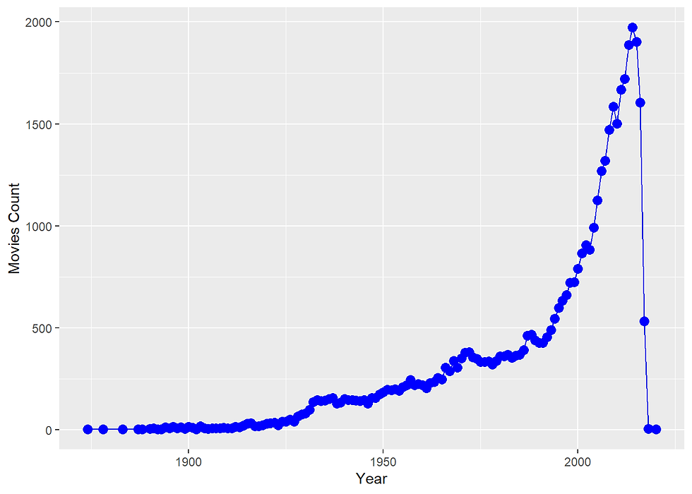 

In Python

df_movies_.loc[:, ‘release_date_’] = pd.to_datetime(df_movies_[‘release_date’], errors=‘coerce’)

ts_movies = df_movies_[“release_date_”].dt.year.value_counts().sort_index()

ax = ts_movies.plot(marker=‘o’)
ax.set_ylabel(‘Movies Count’);
ax.set_xlabel(‘year’);