


Exploring categorical variables (UIC heart disease data)
- sam33frodon
- Dec 28, 2020
- 11 min read
Updated: Dec 30, 2020
data <- read_csv("heart.csv")## Parsed with column specification:
## cols(
## age = col_double(),
## sex = col_double(),
## cp = col_double(),
## trestbps = col_double(),
## chol = col_double(),
## fbs = col_double(),
## restecg = col_double(),
## thalach = col_double(),
## exang = col_double(),
## oldpeak = col_double(),
## slope = col_double(),
## ca = col_double(),
## thal = col_double(),
## target = col_double()
## )
str(data)## Classes 'spec_tbl_df', 'tbl_df', 'tbl' and 'data.frame': 303 obs. of 14 variables:
## $ age : num 63 37 41 56 57 57 56 44 52 57 ...
## $ sex : num 1 1 0 1 0 1 0 1 1 1 ...
## $ cp : num 3 2 1 1 0 0 1 1 2 2 ...
## $ trestbps: num 145 130 130 120 120 140 140 120 172 150 ...
## $ chol : num 233 250 204 236 354 192 294 263 199 168 ...
## $ fbs : num 1 0 0 0 0 0 0 0 1 0 ...
## $ restecg : num 0 1 0 1 1 1 0 1 1 1 ...
## $ thalach : num 150 187 172 178 163 148 153 173 162 174 ...
## $ exang : num 0 0 0 0 1 0 0 0 0 0 ...
## $ oldpeak : num 2.3 3.5 1.4 0.8 0.6 0.4 1.3 0 0.5 1.6 ...
## $ slope : num 0 0 2 2 2 1 1 2 2 2 ...
## $ ca : num 0 0 0 0 0 0 0 0 0 0 ...
## $ thal : num 1 2 2 2 2 1 2 3 3 2 ...
## $ target : num 1 1 1 1 1 1 1 1 1 1 ...
## - attr(*, "spec")=
## .. cols(
## .. age = col_double(),
## .. sex = col_double(),
## .. cp = col_double(),
## .. trestbps = col_double(),
## .. chol = col_double(),
## .. fbs = col_double(),
## .. restecg = col_double(),
## .. thalach = col_double(),
## .. exang = col_double(),
## .. oldpeak = col_double(),
## .. slope = col_double(),
## .. ca = col_double(),
## .. thal = col_double(),
## .. target = col_double()
## .. )The dataset consists of 14 physological patient attributes as follows:
Attribute Information
age: age (continuous)
sex: gender (categorical, 0=male, 1=female)
cp: chest pain type (4 values, ordinal/categorical))
trestbps resting blood pressure (continuous)
chol: serum cholestoral in mg/dl (continuous)
fbs: fasting blood sugar > 120 mg/dl (categorical is >120 =1 or <120 =0)
restecg: resting electrocardiographic results (values 0,1,2, categorical)
thalack: maximum heart rate achieved (continuous)
exang: exercise induced angina (categorical, 1=angina 0 = no agina)
oldpeak: ST depression induced by exercise relative to rest (continuous)
slope: the slope of the peak exercise ST segment (continuous)
ca : number of major vessels (0-3) colored by flourosopy (factor)
thal 3 = normal; 6 = fixed defect; 7 = reversable defect (categorical)
target 1= heart disease present; 0 = no heart disease (categorical, dependant variable)
1. Data engineering
data2 <- data %>%
  mutate(sex = if_else(sex == 1, "MALE", "FEMALE"),
         fbs = if_else(fbs == 1, ">120", "<=120"),
         exang = if_else(exang == 1, "YES" ,"NO"),
         cp = if_else(cp == 1, "ATYPICAL ANGINA",
                      if_else(cp == 2, "NON-ANGINAL PAIN", "ASYMPTOMATIC")),
         restecg = if_else(restecg == 0, "NORMAL",
                           if_else(restecg == 1, "ABNORMALITY", "PROBABLE OR DEFINITE")),
         target = if_else(target == 1, "YES", "NO")
         ) %>%
  mutate_if(is.character, as.factor) %>%
dplyr::select(target, sex, fbs, exang, cp, restecg, slope, ca, thal, everything())str(data2)## Classes 'spec_tbl_df', 'tbl_df', 'tbl' and 'data.frame': 303 obs. of 14 variables:
## $ target : Factor w/ 2 levels "NO","YES": 2 2 2 2 2 2 2 2 2 2 ...
## $ sex : Factor w/ 2 levels "FEMALE","MALE": 2 2 1 2 1 2 1 2 2 2 ...
## $ fbs : Factor w/ 2 levels "<=120",">120": 2 1 1 1 1 1 1 1 2 1 ...
## $ exang : Factor w/ 2 levels "NO","YES": 1 1 1 1 2 1 1 1 1 1 ...
## $ cp : Factor w/ 3 levels "ASYMPTOMATIC",..: 1 3 2 2 1 1 2 2 3 3 ...
## $ restecg : Factor w/ 3 levels "ABNORMALITY",..: 2 1 2 1 1 1 2 1 1 1 ...
## $ slope : num 0 0 2 2 2 1 1 2 2 2 ...
## $ ca : num 0 0 0 0 0 0 0 0 0 0 ...
## $ thal : num 1 2 2 2 2 1 2 3 3 2 ...
## $ age : num 63 37 41 56 57 57 56 44 52 57 ...
## $ trestbps: num 145 130 130 120 120 140 140 120 172 150 ...
## $ chol : num 233 250 204 236 354 192 294 263 199 168 ...
## $ thalach : num 150 187 172 178 163 148 153 173 162 174 ...
## $ oldpeak : num 2.3 3.5 1.4 0.8 0.6 0.4 1.3 0 0.5 1.6 ...cols <- c("slope","ca","thal")
Heart <- data2 %>%
mutate_each_(funs(factor(.)),colsstr(Heart)## Classes 'spec_tbl_df', 'tbl_df', 'tbl' and 'data.frame': 303 obs. of 14 variables:
## $ target : Factor w/ 2 levels "NO","YES": 2 2 2 2 2 2 2 2 2 2 ...
## $ sex : Factor w/ 2 levels "FEMALE","MALE": 2 2 1 2 1 2 1 2 2 2 ...
## $ fbs : Factor w/ 2 levels "<=120",">120": 2 1 1 1 1 1 1 1 2 1 ...
## $ exang : Factor w/ 2 levels "NO","YES": 1 1 1 1 2 1 1 1 1 1 ...
## $ cp : Factor w/ 3 levels "ASYMPTOMATIC",..: 1 3 2 2 1 1 2 2 3 3 ...
## $ restecg : Factor w/ 3 levels "ABNORMALITY",..: 2 1 2 1 1 1 2 1 1 1 ...
## $ slope : Factor w/ 3 levels "0","1","2": 1 1 3 3 3 2 2 3 3 3 ...
## $ ca : Factor w/ 5 levels "0","1","2","3",..: 1 1 1 1 1 1 1 1 1 1 ...
## $ thal : Factor w/ 4 levels "0","1","2","3": 2 3 3 3 3 2 3 4 4 3 ...
## $ age : num 63 37 41 56 57 57 56 44 52 57 ...
## $ trestbps: num 145 130 130 120 120 140 140 120 172 150 ...
## $ chol : num 233 250 204 236 354 192 294 263 199 168 ...
## $ thalach : num 150 187 172 178 163 148 153 173 162 174 ...
## $ oldpeak : num 2.3 3.5 1.4 0.8 0.6 0.4 1.3 0 0.5 1.6 ...Attribute Statistics
Basic statistics about the data are obtained in the below table:
##  target        sex         fbs      exang                    cp
##  NO :138   FEMALE: 96   <=120:258   NO :204   ASYMPTOMATIC    :166
##  YES:165   MALE  :207   >120 : 45   YES: 99   ATYPICAL ANGINA : 50
##                                               NON-ANGINAL PAIN: 87
##
##
##
##                  restecg    slope   ca      thal         age
##  ABNORMALITY         :152   0: 21   0:175   0:  2   Min.   :29.00
##  NORMAL              :147   1:140   1: 65   1: 18   1st Qu.:47.50
##  PROBABLE OR DEFINITE:  4   2:142   2: 38   2:166   Median :55.00
##                                     3: 20   3:117   Mean   :54.37
##                                     4:  5           3rd Qu.:61.00
##                                                     Max.   :77.00
##     trestbps          chol          thalach         oldpeak
##  Min.   : 94.0   Min.   :126.0   Min.   : 71.0   Min.   :0.00
##  1st Qu.:120.0   1st Qu.:211.0   1st Qu.:133.5   1st Qu.:0.00
##  Median :130.0   Median :240.0   Median :153.0   Median :0.80
##  Mean   :131.6   Mean   :246.3   Mean   :149.6   Mean   :1.04
##  3rd Qu.:140.0   3rd Qu.:274.5   3rd Qu.:166.0   3rd Qu.:1.60
##  Max.   :200.0   Max.   :564.0   Max.   :202.0   Max.   :6.20
From the summary, we can conclude there are no common issues with unclean data.
There are no “N/A” values and no negative values where one would not expect to see them.
The summary function in R would show those if they existed in the data.
2. Visual exploration of Categorical Variables
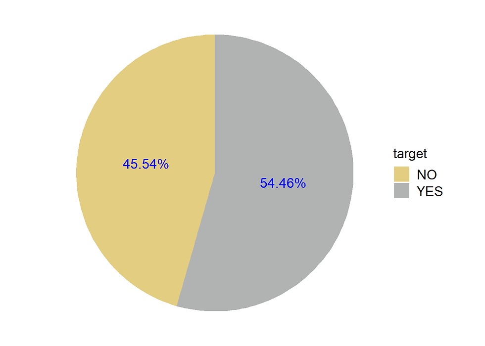
45.54% no heart disease
Heart %>% ggplot(aes(age)) +
  geom_histogram(fill= "lightblue",
                 color = 'blue',
                 binwidth = 1) +
  labs(title= "Age Distribution") +
  theme(plot.title = element_text(hjust = 0.5))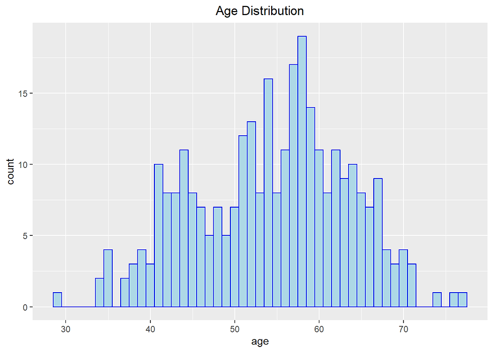
Heart %>% ggplot(aes(age)) +
  geom_histogram(fill= "lightblue",
                 color = 'blue',
                 binwidth = 5) +
  labs(title= "Age Distribution") +
  theme(plot.title = element_text(hjust = 0.5))
Heart %>% ggplot(aes(age)) +
  geom_histogram(aes(fill= target),
                 color = 'grey',
                 binwidth = 1) +
  scale_fill_manual(values=c("#E3CD81FF", "#B1B3B3FF")) +
  labs(title= "Age Distribution for Income")+
  theme(plot.title = element_text(hjust = 0.5))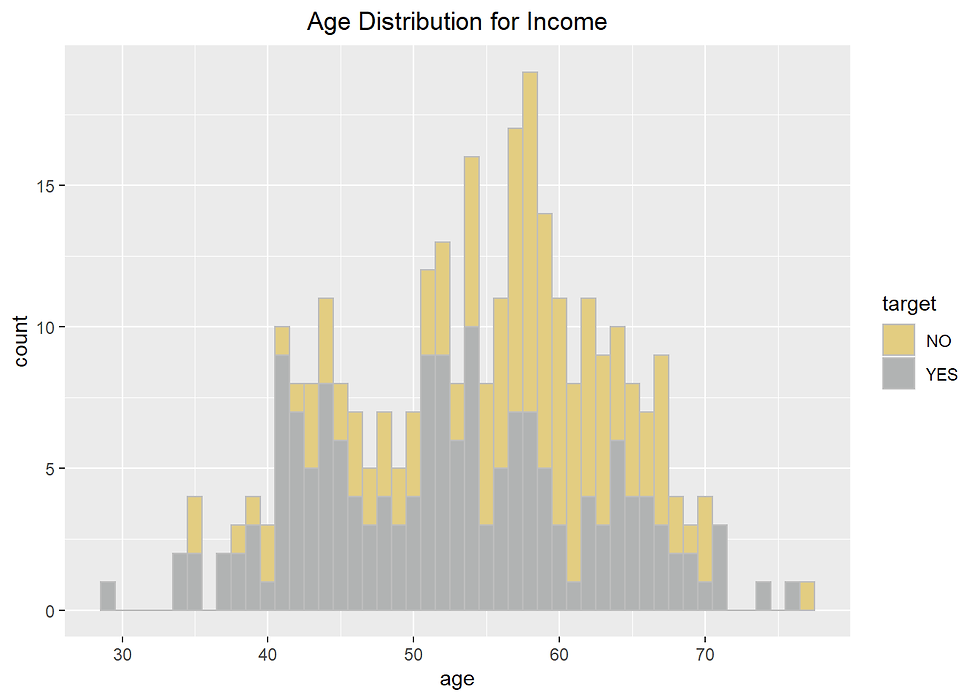
Heart %>%
  ggplot(aes(age,
             fill= target)) +
  geom_density(alpha= 0.7, color = 'blue') +
  scale_fill_manual(values=c("#E3CD81FF", "#B1B3B3FF")) +
  labs(x = "Age", y = "Density", title = "Density graph of age distribution")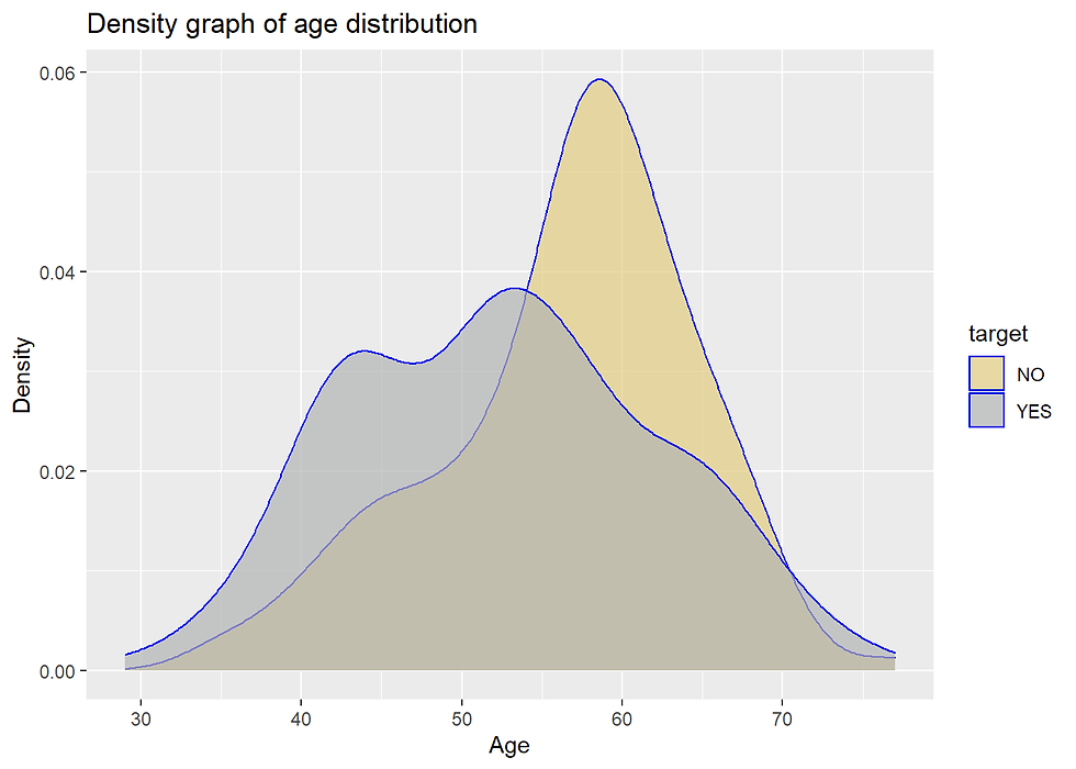
GENDER
library(ggpubr)library(scales)gender_prop <- Heart %>%
group_by(sex) %>%
summarise(count = n()) %>%
ungroup()%>%
arrange(desc(sex)) %>%
mutate(percentage = round(count/sum(count),4)*100,
lab.pos = cumsum(percentage)-0.5*percentage)
gender_distr <- ggplot(data = gender_prop,
aes(x = "",
y = percentage,
fill = sex))+
geom_bar(stat = "identity")+
coord_polar("y") +
geom_text(aes(y = lab.pos,
label = paste(percentage,"%", sep = "")), col = "blue", size = 4) +
scale_fill_manual(values=c("orange", "lightblue"),
name = "Gender") +
theme_void() +
theme(legend.title = element_text(color = "black", size = 12),
legend.text = element_text(color = "black", size = 12))
gender_prop <- Heart %>%
group_by(sex, target) %>%
summarize(n = n()) %>%
mutate(pct = n*100/sum(n)) %>%
ggplot(aes(x = reorder(sex, n),
y = pct,
fill = target)) +
geom_bar(stat = "identity", width = 0.6) +
scale_x_discrete(name = "") +
scale_fill_manual(values=c("#E3CD81FF", "#B1B3B3FF")) +
geom_text(aes(label = paste0(round(pct,0),"%")),
position = position_stack(vjust = 0.5),
size = 4,
color = "black") +
theme(axis.text.y = element_blank(),
axis.text.x = element_text(color = "black", size = 12),
axis.title.y = element_blank(),
axis.ticks.y = element_blank(),
legend.title = element_text(color = "black", size = 12),
legend.text = element_text(color = "black", size = 12))
ggarrange(gender_distr, gender_prop, nrow = 1)
31.68 % of people are male 68.32 % are female
75% of males had heart disease. 45% of female had heart disease.
Distribution of Male and Female population across Age parameter
Heart %>%
  ggplot(aes(x=age,fill=sex))+
  geom_histogram()+
  xlab("Age") +
  ylab("Number")+
  scale_fill_manual(values=c("orange", "lightblue"),
name = "Gender") 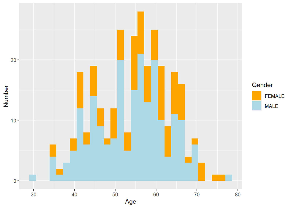
Chest pain type (cp)
cp_distr <- Heart %>%
  group_by(cp) %>%
  summarise(counts = n()) %>%
  mutate(Percentage = round(counts*100/sum(counts),2)) %>%
  arrange(desc(counts)) %>%
  ggplot(aes(x= reorder(cp, counts),
             y  = counts)) +
  geom_bar(stat = "identity",
           width = 0.6,
           fill = "steelblue") +
  geom_text(aes(label = paste0(round(counts,1),"\n",Percentage,"%")),
            vjust = 0.5,
            hjust = -0.5,
            color = "darkblue",
            size = 4) +
  scale_y_continuous(limits = c(0,200)) +
  theme_minimal() +
  labs(x = "Chest pain types",y = "Frequency") +
  coord_flip()

cp_prop <- Heart %>%
  group_by(cp, target) %>%
  summarize(n = n()) %>%
  mutate(pct = n*100/sum(n)) %>%
  ggplot(aes(x = reorder(cp, n),
             y = pct/100,
             fill = target)) +
  geom_bar(stat = "identity", width = 0.6) +
  scale_x_discrete(name = "") +
  scale_y_continuous(name= "Percentage",
                     labels = percent) +
  scale_fill_manual(values=c("#E3CD81FF", "#B1B3B3FF")) +
  geom_text(aes(label = paste0(round(pct,0),"%")),
            position = position_stack(vjust = 0.5),
            size = 4,
            color = "black") +
  theme(plot.title = element_text(hjust = 0.5),
        axis.text.y=element_blank()) +
  coord_flip()

ggarrange(cp_distr, cp_prop, nrow = 1)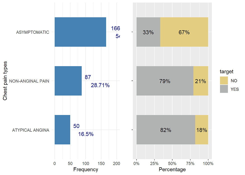
Fasting blood sugar (fbs)
fbs_distr <- Heart %>%
  group_by(fbs) %>%
  dplyr::summarise(counts = n()) %>%
  mutate(Percentage = round(counts*100/sum(counts),2)) %>%
  arrange(desc(counts)) %>%
  ggplot(aes(x= reorder(fbs, counts),
             y  = counts)) +
  geom_bar(stat = "identity",
           width = 0.6,
           fill = "steelblue") +
  geom_text(aes(label = paste0(round(counts,1),"\n",Percentage,"%")),
            vjust = 0.5,
            hjust = -0.5,
            color = "darkblue",
            size = 4) +
  scale_y_continuous(limits = c(0,350)) +
  theme_minimal() +
  labs(x = "Chest pain types",y = "Frequency") +
  coord_flip()

fbs_prop <- Heart %>%
  group_by(fbs, target) %>%
  dplyr::summarize(n = n()) %>%
  mutate(pct = n*100/sum(n)) %>%
  ggplot(aes(x = reorder(fbs, n),
             y = pct/100,
             fill = target)) +
  geom_bar(stat = "identity", width = 0.6) +
  scale_x_discrete(name = "") +
  scale_y_continuous(name= "Percentage",
                     labels = percent) +
  scale_fill_manual(values=c("#E3CD81FF", "#B1B3B3FF")) +
  geom_text(aes(label = paste0(round(pct,0),"%")),
            position = position_stack(vjust = 0.5),
            size = 4,
            color = "black") +
  theme(plot.title = element_text(hjust = 0.5),
        axis.text.y=element_blank()) +
  coord_flip()

ggarrange(fbs_distr,fbs_prop, nrow = 1)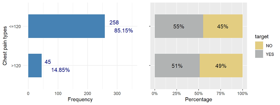
It seems that there is a slight difference in percentage of pp having heart disease for two groups (fasting blood sugar)
chisq.test(Heart$target, Heart$fbs)##
## Pearson's Chi-squared test with Yates' continuity correction
##
## data: Heart$target and Heart$fbs
## X-squared = 0.10627, df = 1, p-value = 0.7444The p = 0.744 > 0.05. There is no relationship between fast blood sugar and heart disease for this data.
restecg resting electrocardiographic results (values 0,1,2, categorical)
restecg_distr <- Heart %>%
  group_by(restecg) %>%
  dplyr::summarise(counts = n()) %>%
  mutate(Percentage = round(counts*100/sum(counts),2)) %>%
  arrange(desc(counts)) %>%
  ggplot(aes(x= restecg,
             y  = counts)) +
  geom_bar(stat = "identity",
           width = 0.6,
           fill = "steelblue") +
  geom_text(aes(label = paste0(round(counts,1),"\n",Percentage,"%")),
            vjust = 0.5,
            hjust = -0.5,
            color = "darkblue",
            size = 4) +
  scale_y_continuous(limits = c(0,250)) +
  theme_minimal() +
  labs(x = "resting electrocardiographic results",y = "Frequency") +
  coord_flip()

restecg_prop <- Heart %>%
  group_by(restecg, target) %>%
  dplyr::summarize(n = n()) %>%
  mutate(pct = n*100/sum(n)) %>%
  ggplot(aes(x = restecg,
             y = pct/100,
             fill = target)) +
  geom_bar(stat = "identity", width = 0.6) +
  scale_x_discrete(name = "") +
  scale_y_continuous(name= "Percentage",
                     labels = percent) +
  scale_fill_manual(values=c("#E3CD81FF", "#B1B3B3FF")) +
  geom_text(aes(label = paste0(round(pct,0),"%")),
            position = position_stack(vjust = 0.5),
            size = 4,
            color = "black") +
  theme(plot.title = element_text(hjust = 0.5),
        axis.text.y=element_blank()) +
  coord_flip()

ggarrange(restecg_distr,restecg_prop, nrow = 1)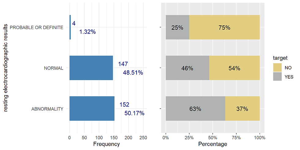
chisq.test(data$target, Heart$restecg)## Warning in chisq.test(data$target, Heart$restecg): Chi-squared approximation may
## be incorrect##
## Pearson's Chi-squared test
##
## data: data$target and Heart$restecg
## X-squared = 10.023, df = 2, p-value = 0.006661exang exercise induced angina (categorical, 1=angina 0 = no agina)
Angina (pronounced ANN-juh-nuh or ann-JIE-nuh) is pain in the chest that comes on with exercise, stress, or other things that make the heart work harder.
exang_distr <- Heart %>%
  group_by(exang) %>%
  dplyr::summarise(counts = n()) %>%
  mutate(Percentage = round(counts*100/sum(counts),2)) %>%
  arrange(desc(counts)) %>%
  ggplot(aes(x= exang,
             y  = counts)) +
  geom_bar(stat = "identity",
           width = 0.6,
           fill = "steelblue") +
  geom_text(aes(label = paste0(round(counts,1),"\n",Percentage,"%")),
            vjust = 0.5,
            hjust = -0.5,
            color = "darkblue",
            size = 4) +
  scale_y_continuous(limits = c(0,300)) +
  theme_minimal() +
  labs(x = "Exercise induced anginas",y = "Frequency") +
  coord_flip()

exang_prop <- Heart %>%
  group_by(exang, target) %>%
  dplyr::summarize(n = n()) %>%
  mutate(pct = n*100/sum(n)) %>%
  ggplot(aes(x = exang,
             y = pct/100,
             fill = target)) +
  geom_bar(stat = "identity", width = 0.6) +
  scale_x_discrete(name = "") +
  scale_y_continuous(name= "Percentage",
                     labels = percent) +
  scale_fill_manual(values=c("#E3CD81FF", "#B1B3B3FF")) +
  geom_text(aes(label = paste0(round(pct,0),"%")),
            position = position_stack(vjust = 0.5),
            size = 4,
            color = "black") +
  theme(plot.title = element_text(hjust = 0.5),
        axis.text.y=element_blank()) +
  coord_flip()

ggarrange(exang_distr,exang_prop, nrow = 1)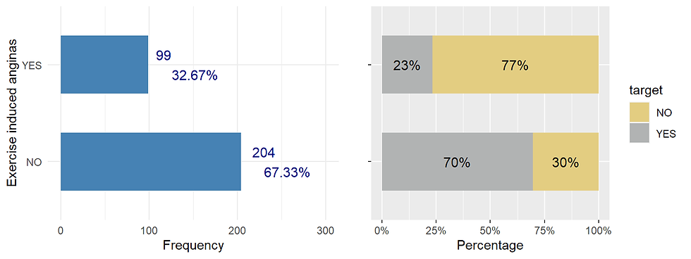
ca number of major vessels (0-3) colored by flourosopy (factor)
ca_distr <- Heart %>%
  group_by(ca) %>%
  dplyr::summarise(counts = n()) %>%
  mutate(Percentage = round(counts*100/sum(counts),2)) %>%
  arrange(desc(counts)) %>%
  ggplot(aes(x= ca,
             y  = counts)) +
  geom_bar(stat = "identity",
           width = 0.6,
           fill = "steelblue") +
  geom_text(aes(label = paste0(round(counts,1),"\n",Percentage,"%")),
            vjust = 0.5,
            hjust = -0.5,
            color = "darkblue",
            size = 4) +
  scale_y_continuous(limits = c(0,300)) +
  theme_minimal() +
  labs(x = "Number of major vessels colored by fluoroscopy",y = "Frequency") +
  coord_flip()

ca_prop <- Heart %>%
  group_by(ca, target) %>%
  dplyr::summarize(n = n()) %>%
  mutate(pct = n*100/sum(n)) %>%
  ggplot(aes(x = ca,
             y = pct/100,
             fill = target)) +
  geom_bar(stat = "identity", width = 0.6) +
  scale_x_discrete(name = "") +
  scale_y_continuous(name= "Percentage",
                     labels = percent) +
  scale_fill_manual(values=c("#E3CD81FF", "#B1B3B3FF")) +
  geom_text(aes(label = paste0(round(pct,0),"%")),
            position = position_stack(vjust = 0.5),
            size = 4,
            color = "black") +
  theme(plot.title = element_text(hjust = 0.5),
        axis.text.y=element_blank()) +
  coord_flip()

ggarrange(ca_distr,ca_prop, nrow = 1)
thal
thal_distr <- Heart %>%
  group_by(thal ) %>%
  dplyr::summarise(counts = n()) %>%
  mutate(Percentage = round(counts*100/sum(counts),2)) %>%
  arrange(desc(counts)) %>%
  ggplot(aes(x= thal ,
             y  = counts)) +
  geom_bar(stat = "identity",
           width = 0.6,
           fill = "steelblue") +
  geom_text(aes(label = paste0(round(counts,1),"\n",Percentage,"%")),
            vjust = 0.5,
            hjust = -0.5,
            color = "darkblue",
            size = 4) +
  scale_y_continuous(limits = c(0,300)) +
  theme_minimal() +
  labs(x = "Thalium stress test result",y = "Frequency") +
  coord_flip()

thal_prop <- Heart %>%
  group_by(thal , target) %>%
  dplyr::summarize(n = n()) %>%
  mutate(pct = n*100/sum(n)) %>%
  ggplot(aes(x = thal ,
             y = pct/100,
             fill = target)) +
  geom_bar(stat = "identity", width = 0.6) +
  scale_x_discrete(name = "") +
  scale_y_continuous(name= "Percentage",
                     labels = percent) +
  scale_fill_manual(values=c("#E3CD81FF", "#B1B3B3FF")) +
  geom_text(aes(label = paste0(round(pct,0),"%")),
            position = position_stack(vjust = 0.5),
            size = 4,
            color = "black") +
  theme(plot.title = element_text(hjust = 0.5),
        axis.text.y=element_blank()) +
  coord_flip()

ggarrange(thal_distr,thal_prop, nrow = 1)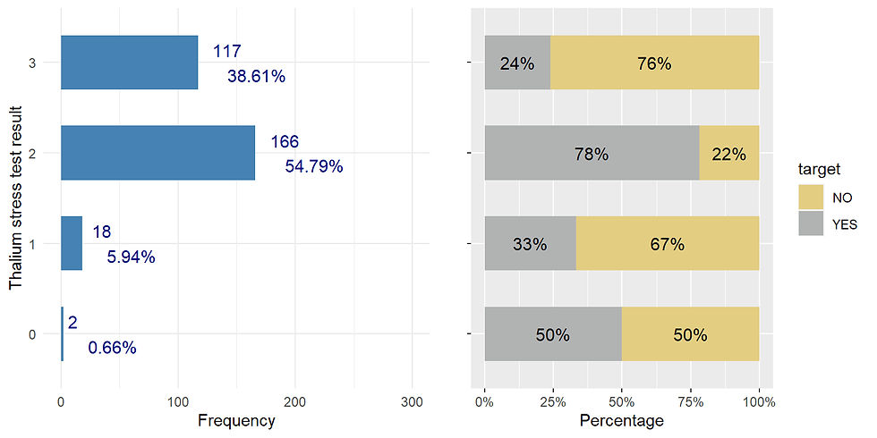
exercise ST segment (upsloping, flat, or downsloping
slope_distr <- Heart %>%
  group_by(slope) %>%
  dplyr::summarise(counts = n()) %>%
  mutate(Percentage = round(counts*100/sum(counts),2)) %>%
  arrange(desc(counts)) %>%
  ggplot(aes(x= slope,
             y  = counts)) +
  geom_bar(stat = "identity",
           width = 0.4,
           fill = "steelblue") +
  geom_text(aes(label = paste0(round(counts,1),"\n",Percentage,"%")),
            vjust = 0.5,
            hjust = -0.5,
            color = "darkblue",
            size = 4) +
  scale_y_continuous(limits = c(0,200)) +
  theme_minimal() +
  labs(x = "Slope of peak exercise ST segment",y = "Frequency") +
  coord_flip()

slope_prop <- Heart %>%
  group_by(slope, target) %>%
  dplyr::summarize(n = n()) %>%
  mutate(pct = n*100/sum(n)) %>%
  ggplot(aes(x = slope,
             y = pct/100,
             fill = target)) +
  geom_bar(stat = "identity", width = 0.6) +
  scale_x_discrete(name = "") +
  scale_y_continuous(name= "Percentage",
                     labels = percent) +
  scale_fill_manual(values=c("#E3CD81FF", "#B1B3B3FF")) +
  geom_text(aes(label = paste0(round(pct,0),"%")),
            position = position_stack(vjust = 0.5),
            size = 4,
            color = "black") +
  theme(plot.title = element_text(hjust = 0.5),
        axis.text.y=element_blank()) +
  coord_flip()

ggarrange(slope_distr,slope_prop, nrow = 1)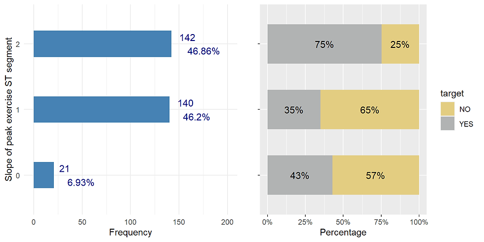
Numerical variable trestbps Resting blood pressure (mm Hg)
Heart %>% ggplot(aes(trestbps)) +
  geom_histogram(fill= "lightblue",
                 color = 'blue',
                 binwidth = 1) +
  labs(title= "Resting blood pressure") +
  theme(plot.title = element_text(hjust = 0.5))
Heart %>%
  ggplot(aes(trestbps,
             fill= target)) +
  geom_density(alpha= 0.7, color = 'blue') +
  scale_fill_manual(values=c("#E3CD81FF", "#B1B3B3FF")) +
  labs(x = "Age", y = "Density", title = "Density graph of trestbps distribution")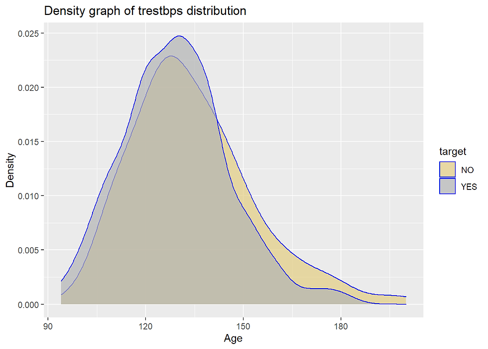
chol Serum cholesterol (mg/dl)
Heart %>% ggplot(aes(chol)) +
  geom_histogram(fill= "lightblue",
                 color = 'blue',
                 binwidth = 3) +
  labs(title= "Serum cholesterol (mg/dl)") +
  theme(plot.title = element_text(hjust = 0.5))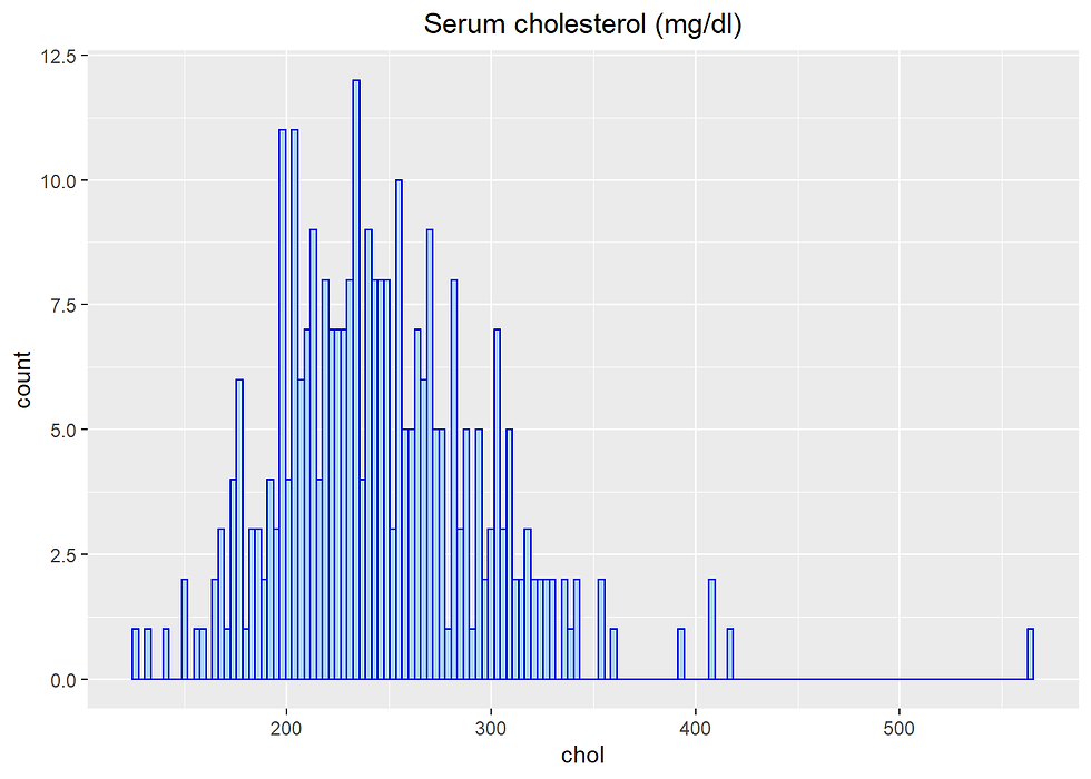
To be continued.


Comments